Introduction

Historically, much of the improvement in computer performance has been driven by improvements in the underlying hardware. Programmers who had performance issues could just wait for newer processors to come out with smaller transistors or faster clock speeds, and their problems would be solved. Unfortunately, Moore’s law has slowed down, and with it yearly single-threaded performance gains have also slowed. Worse, new workloads such as computer vision, simulation, or AI have created an unprecedented demand for compute power. If programmers can no longer scale up their hardware solutions, another option is to scale out by parallelizing the work. Although it is more difficult to program, many tasks can be broken down into chunks that can be executed in parallel. By parallelizing their execution strategies, dramatic performance improvements can be realized.

This post considers a classical problem in computer vision: the computation of a disparity map. This computation, which is a key element of the algorithm which transforms a pair of images acquired from a stereo camera into an ordered point cloud, is both computationally heavy and parallelizable. In this post, we implement this algorithm with multiple parallelization strategies. Beginning with no parallization, we explore parallizing via multithreading via the OpenMP library, using Single Instruction Multiple Data (SIMD) instructions, and finally using special-purpose parallel compute hardware in the form of NVIDIA GPUs via the CUDA and OpenCL frameworks. In addition to benchmarking the algorithms against each other, this post discusses the benefits and drawbacks of each of the different algorithms, and what sorts of problems they lend themselves well towards solving. The code has been uploaded to Github; the link can be found at the bottom of this post.

Theory

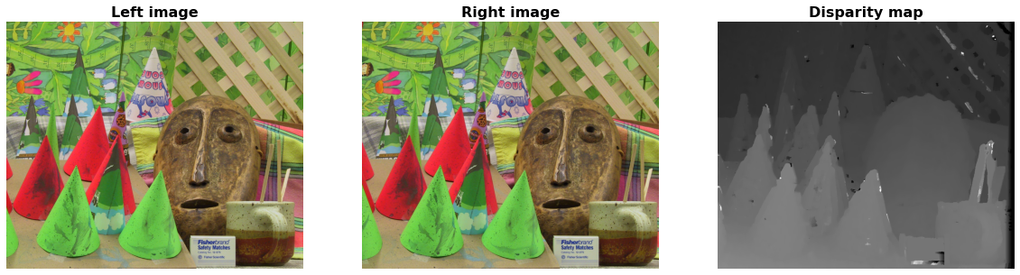
One mechanism for computing depth from a pair of images in a stereo camera involves matching each pixel in the image from the left camera with the corresponding pixel in the right camera. The further apart the pixels are in terms of X-Y coordinates, the closer the object is to the camera. A disparity map is a data structure that records this distance for each pixel. An example of a disparity map is shown below. Given the left and the right image, the computed disparity map is shown on the right. Pixels with larger disparity values are shown in a lighter color. We can see that the objects that are closer to the image are lighter in color, matching our assumption.

One of the simplest ways to compute this value is via an algorithm called “block matching.” In this algorithm, a square “neighborhood” is considered around each pixel. This “block” is then compared at various points in each image, and a loss function is computed for each candidate. This loss function will be zero if an exact match is found. In most cases, however, an exact match will not be found, due to minor variations in illumination, occlusion, or a variety of other reasons. If an exact match is not found, the pixel’s position can be estimated with sub-pixel accuracy by fitting a parabola to the three closest matching points.

The description above describes a generic formula, of which there are countless variations. For more information on the how to compute the disparity map, consult Chris McCormick’s excellent blog post on the topic or an excellent Matlab tutorial on the topic. For the purposes of this blog post, we will make the following assumptions:

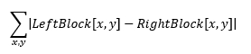
• The disparity metric that we will use will be the Sum of Absolute Differences, which can be expressed by the following formula:
  
• We will assume that the images are stereo-rectified, so that the best matching pixel in the right image will have the same Y coordinate and an X coordinate that is greater than or equal to the best matching pixel in the left image.

With these assumptions, our algorithm can be described by the following pseudocode:

ComputeDisparity:
  Input:  ImageL
  Input:  ImageR
  Input:  BlockSize # Size of the neighborhood to consider
  Input:  ScanSize  # Number of neighboring blocks to consider
  Output: Disparity

  For each Y,X in ImageL: #(A)
    Compute the template size, taking edges into account
    Compute the number of candidate pixels, taking edges into account
    Losses = []
    For each candidate pixel: #(B)
      Compute Disparity Metric over candidate pixel neighborhood and root neighborhood #(C)
      Append Disparity Matric to Losses

    BestIndex = argmin(losses)

    # Compute disparity to subpixel accuracy
    A = losses[BestIndex-1]
    B = losses[BestIndex]
    C = losses[BestIndex+1]
    Parabola = FitParabola((-1, A), (0, B), (1, C))
    (P_X, P_Y) = Minimize(Parabola)
    D = BestIndex + P_X

    Disparity[X,Y] = D

Baseline Implementation

The algorithm described in pseudocode above has been implemented in this c++ class. This class, like all others discussed in the post, accepts two grayscale images and returns a disparity map. We can run it through a simple benchmark with the following parameters:

• CPU: Intel i7-4790, clocked at 4 GHz
• RAM: 32 GB, DDR3
• Compiler: Clang 9.0.0
• Compiler flags: -O3 -fopenmp -march=native -stc=c++17
• GPU: NVidia GTX970
• CUDA: version 10.2
• Image size: 750x900
• Block Size: 15
• Scan size: 50
• 1100 iterations, discard first 100

The benchmarking code is here. The resulting performance looks like this:

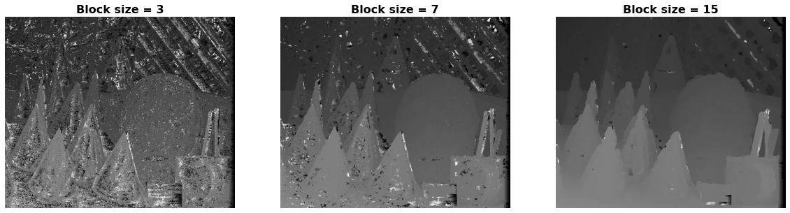
This single-threaded implementation takes over 3 seconds to compute the disparity map! By analyzing the pseudocode above, we can see that the computational complexity of this algorithm is O(Image_Width * Image_Height * Scan_Size * Block_Width * Block_Height). Typically, large images are used in order to increase the resolution of the sensor. It is also desirable to consider a large number of candidate regions, in order to allow the sensor to accurately detect distances both near and far away. Finally, large neighborhoods are typically used in order to avoid artifacts. Shown below is the same algorithm run with block sizes of 7, 15, and 23 pixels. Notice how increasing the block size smoothes out the disparity map computation.

Although there are some algorithmic tricks that can be used to improve the performance of the algorithm (e.g. pyramiding), they will not be considered in this this post. Instead, we’ll take advantage of the fact that there are multiple opportunities to inject parallelism into the algorithm:

• The disparity for each pixel can be computed independently of each other. This is marked at point (A) in the pseudocode.
• For each pixel, the disparity of each of the candidates can be computed independently. This is marked at point (B) in the pseudocode.
• The SAD value for each pair of pixels in the neighborhood can be computed independently. This is marked at point (C) in the pseudocode.

Threads

Modern processors typically have multiple cores, each of which is capable of executing a single series of instructions, called a “thread.” By default, processes use a single thread for their computation, but they can spawn more. By spawning more threads, the program can use more cores, scaling out the compute job. Multi-threaded programming is much more difficult than single-threaded programming, but it can lead to massive performance gains if the problem is parallelizable.

Many modern compilers, such as clang and gcc, implement the OpenMP featureset. OpenMP allows one to parallelize computation across multiple threads via special compiler pragmas. This hides the complexity of managing threads from the application, allowing the developer to focus on writing application logic. In particular, the macro of interest here is #pramga omp parallel for. When applied to a simple for loop, this pragma parallelizes it across many threads, speeding up execution dramatically. We can attempt to parallelize the three for loops in the above algorithm using OpenMP, with the following results:

• Point A: Runtime is about 1 second, a good speedup over the single threaded program.
• Point B: Runtime is about 3 seconds, about the same as the single threaded program.
• Point C: Runtime is about 2 minutes, a huge slowdown over the single threaded program.

We see a huge performance improvement when we parallize at point (A), a less important one at (B), and a huge performance decrease at point (C). The reason (B) and (C) don’t help much is that there is an overhead to spawning and destroying threads. If there is not much work to be done on each thread, then the cost of spawning the thread outweights the gain from parallelizing. In addition, if multiple for loops are parallelized in this manner, then the system will become overloaded with threads, and performance will not be improved.

Up until this point, the benchmarks have only been considering “Wall clock time”, or the time measured in the real world. Another way of measuring performance is CPU time, which is the amount of time a CPU is actively processing a task. For a single-threaded task that is never switched off a core, these two measures are equivalent, but for a multi-threaded program, they can be drastically different:

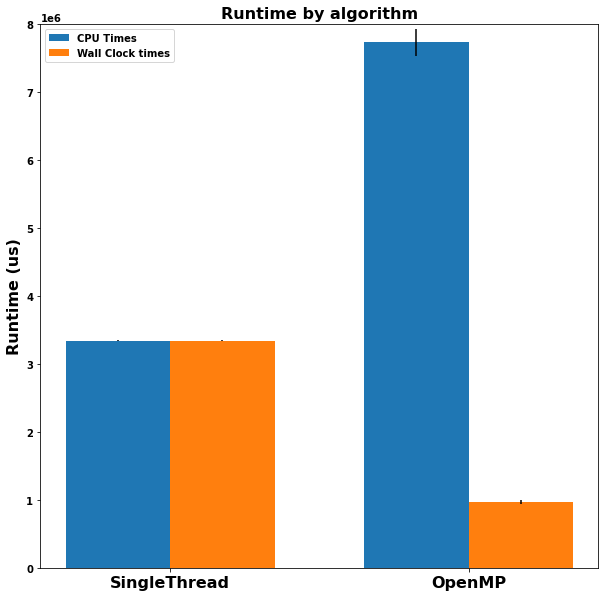
Here, we see that while using OpenMP decreased the wall clock time significantly, it drastically increased the CPU time! This makes sense because the algorithm is using an enormous amount of system resources to run. The image below shows two snapshots of the CPU state. The first one is the CPU state when the single-threaded algorithm is running:

This one is when the OpenMP algorithm is running.

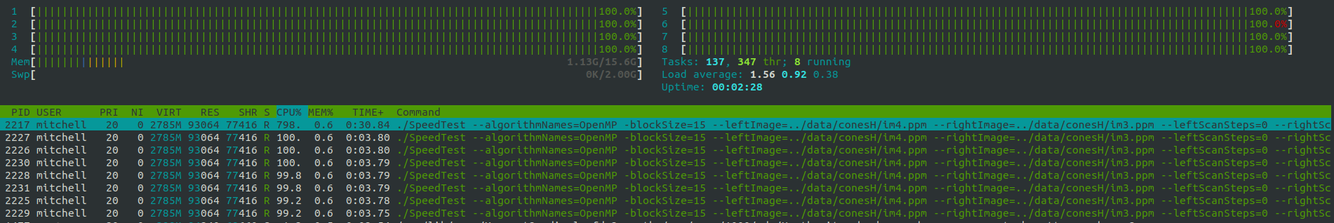
The OpenMP algorithm is using 8x the system resources! This could rule out threading as a means of parallelization if the CPU is already under a heavy load or needs to run other applications.

SIMD Instructions

Typically, each CPU instruction performs an operation on a single piece of data. For exaple, an “ADD” instruction might add two integers together and store the result in a register. These instructions are called “Single instruction, Single Data” instructions. Some workloads, however, perform the exact same operations on multiple pieces of data. For example, computing when computing the dot product of two vectors, the same mathematical operations are called on each element of the vector independently of the others. In order to take advantage of this parallelism, CPU designers have designed instructions that can perform identical operations on multiple pieces of data, called “Single Insruction, Multiple Data” or “SIMD” instructions. For example, a SIMD Add instruction might compute the sum of 8 integers in parallel. SIMD workloads are a more efficient method of parallelization than threads because they decrease the number of operations the computer needs to perform. However, they are more difficult to write, and they are less flexible than threading because they require the exact same operations to be performed on each piece of data. Conditionals and control flow are difficult to perform with most SIMD instruction sets.

For the disparity map computation, the computation of the disparity metric is a great candidate for employing SIMD instructions. A simple implementation without using SIMD might look like this:

int sum = 0;
for (int y = 0; y < height; y++) {
    for (int x = 0; x < width; x++) {
        sum += std::abs(
            leftImage.at<unsigned char>(y + minYL, x + minXL)
            - rightImage.at<unsigned char>(y + minYR, x + minXR));
    }
}
return sum;

A functionally equivalent SIMD transformation might look like this:

// Declare the special SIMD memory registers
// __m256i means a 256-bit register formed from 8 integers
union { __m256i accumulator; uint64_t accumulatorValues[4]; };
union { __m256i workRegA; uint8_t workRegABytes[32]; };
union { __m256i workRegB; uint8_t workRegBBytes[32]; };
union { __m256i maskReg; uint8_t maskRegBytes[32]; };
union { __m256i sadReg; uint8_t sadRegBytes[32]; };

// Initialize the accumulators
__m256i zeros;
accumulator = _mm256_setzero_si256();
maskReg = _mm256_setzero_si256();
zeros = _mm256_setzero_si256();

uint8_t* leftImageData = leftImage.data;
uint8_t* rightImageData = rightImage.data;

// Because each SIMD operation works on 32 integers, 
//   mask out the bytes outside the respective windows
for (int i = 0; i < width; i++) {
    maskRegBytes[i] = 0xFF;
}

// The main loop performing work
// Notice how this now only goes over Y, not Y and X
for (int y = 0; y < height; y++) {
    // Load the data into the SIMD registers
    int leftLoadIdx = (leftImage.cols * (y+minYL)) + minXL;
    int rightLoadIdx = (rightImage.cols * (y+minYR)) + minXR;
    workRegA = _mm256_loadu_si256(
        reinterpret_cast<__m256i const*>(leftImageData + leftLoadIdx));
    workRegB = _mm256_loadu_si256(
        reinterpret_cast<__m256i const*>(rightImageData + rightLoadIdx));

    // First, mask out the bytes that are outside the window bounds with the blendv instruction
    // Then, use the SAD instruction to compute the SAD metric
    sadReg = _mm256_sad_epu8(
            _mm256_blendv_epi8(zeros, workRegA, maskReg),
            _mm256_blendv_epi8(zeros, workRegB, maskReg)
            );
           
    // sad_epu8 stores the results as 4 16-bit integers.
    // Add them to the accumulator values.
    accumulator = _mm256_add_epi64(sadReg, accumulator);
}

// The results are stored as 4 separate integers,
// Sum them up to get the total result.
int result = 0;
for (int i = 0; i < 4; i++) {
    result += static_cast<int>(accumulatorValues[i]);
}

return result;

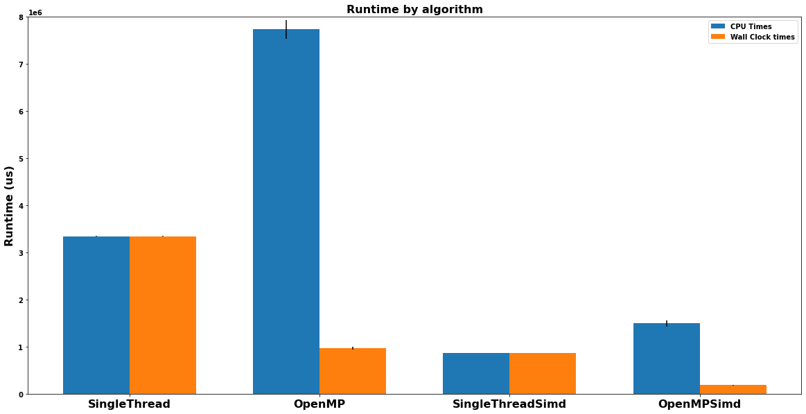
While this looks more complicated, the net effect is that the nested for loop has been reduced to a single for loop, with each of the computations being performed in parallel. This has a dramatic effect on performance, decreasing both the wall-clock and CPU-clock time it takes for the computation to run. In addition, this method can be combined with threading to further improve performance. The chart below shows a performance comparison of the different algorithms.

GPU compute

Although the parallelization methods above are handy, they are constrained by the fact that modern CPUs generally only have the capability of running a few (i.e. <50) threads simultaneously. This limitation prevents trully parallel workloads from scaling out to their full potential. A variety of computing hardware has been developed which allows for more threads to be run in parallel, the most popular of which is known as a “Graphics Processing Unit,” or GPU. GPUs are designed for graphical applications, in which thousands of threads are run in parallel. Although the computing capabilities of each individual thread is more limited (e.g. fewer specialized instructions are available), the benefit gained from scaling out can be massive.

There are two common ways to use GPUs. The first one is by using a vendor-specific API. For NVIDIA GPUs, the most popular method for running parallel algorithms is via the CUDA API. CUDA code looks very similar to standard C code, with a few minor differences:

• Users specify that code either runs on the “host” (i.e. the controlling PC), the “device” (i.e. the GPU itself), or both.
• Users need to handle copying data to and from the GPU, as well as synchronizing the state of the host and the GPU.
• Some advanced C features are not available.

A sample implementation of the cuda functions used to compute the disparity map can be found in this source file. When using CUDA to parallelize the computation, we can see that the performance improves dramatically:

While CUDA is simple to use and ergonomic, it is only available for NVIDIA GPUs. Each GPU vendor has its own vendor-specific API that can be used. In addition, many GPUs (and other parallel hardware accelerators) support the OpenCL programming specification. OpenCL is a specification that provides a generalized interface to heterogeneous compute hardware. There are some benefits to using OpenCL when programming:

• Platform Independence: After writing a program using the OpenCL API, it should be able to run on any device that supports the OpenCL interface. For example, the same program could run on both CPUs and GPUs. This can be handy, for example, when deploying a program to users who may have a variety of hardware enabled. The program can fall back to the CPU if the GPU is not available.
• Dynamic Execution: With OpenCL, a program can be loaded and compiled dynamically at runtime. This can enable the creation of more generic programs that are specialized at runtime.

There are some important drawbacks, however:

• Difficulty of use: It is difficult to write programs using OpenCL - there are many more details and concepts for the programmer to keep in mind. This leads to a larger volume of code that is more difficult to maintain.
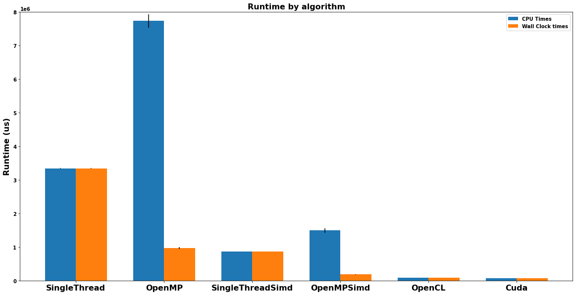
• Performance: Because it’s more generic, most OpenCL APIs are slower than their native counterparts. Shown below is a performance comparison of CUDA and OpenCL. Although the OpenCL implementation is almost identical, it is slightly slower than the CUDA implementation.

Additional Comments

Just like CPUs GPUs also have SIMD instruction sets. However, the instructions that are available are much more limited and less useful. For example, instead of being able to compute the SAD on 32 integers in parallel, the closest analog in CUDA uses 4 bytes that need to be packed inside an unsigned integer. Due to all the additional shuffling, using the SIMD instructions in the CUDA kernel did not significantly improve the runtime.

Parallel programs are difficult to implement, and even more difficult to debug. Before experimenting with parallelization, it is recommended to start with a fully-functional single-threaded implementation that can be used as a reference.

Summary

In this experiment, a simple algorithm for computing the disparity map from a pair of images was developed. The algorithm was implemented using a variety of parallelization frameworks, each with varying effects on the CPU usage and runtime. Each of the different parallelization methods have their use case:

• Single threaded implementations are the simplest to maintain, although the slowest of the bunch.
• Multi threaded implementations trade CPU cycles for wall clock runtime by spreading the work across multiple CPU cores. By using the OpenMP framework, embarrassingly parallel workloads can easily be transformed into multi-threaded parallel programs with a series of compile-time macros.
• SIMD instructions are useful for creating more efficient programs when the exact same series of instructions are performed on multiple pieces of data. Although they are inflexible and difficult to use correctly, the payoff for correctly using these instructions can be massive.
• GPUs can massively speed up parallel workloads, but may not always be available.

Download Links

The code for the experiments can be found here on github.