Introduction

Modern computers contain billions of discrete logic gates. These gates take two binary signals as input, and apply a simple logical rule to compute their output. By combining many of these logic gates into a single circuit, complex logical expressions can be created, which are necessary to allow computers to perform computations that are needed to solve real-world problems. Most commercially-sold processors use a fixed set of gates to perform their computations. At design time, designers map logic gates onto different parts of the silicon. When the chip is fabricated, each of the logic gates are “hard-coded” to perform one specific function. While fixing the functionality of the gates simplifies design and fabrication, one might ask if it is possible to create a configurable logic gate, that is possible to be reconfigured on the fly. This would have numerous benefits to the end-user, potentially decreasing chip size, decreasing power usage, and increasing resiliency of the hardware to failures.

One potential mechanism for creating these reconfigurable hardware blocks, or “universal gates”, is via leveraging the power of chaotic functions. Chaotic functions are functions that satisfy two desirable properties. First, chaotic functions are deterministic, meaning that given a fixed set of inputs, the function will always compute the same output. Chaotic functions are also sensitive to their initial conditions, meaning that changing the inputs slightly changes the output dramatically. Both properties are necessary to create a universal gate. Without determinisim, it is impossible to reproduce the output. Without sensitivity to initial conditions, it is difficult to get the variety of behavior necessary to create the universal gate.

An interesting series of papers by Ditto and Sinha propose a framework for using chaotic functions to build a universal gate. In this post, we will dive into the content of these papers with the intent of implementing them on an FPGA. Along the way, we will make some improvements to the algorithm for implementation on a digital platform, as well as discover some unsolved problems with their approach. Finally, we will implement the universal gate on an FPGA, and use them to build a morphable computer that can swap between performing the functions of addition and multiplication for 2-bit inputs.

Motivation

Currently, most computer chips have a relatively small number of “cores”, or hard-wired set of logic gates that perform general computation. For example, a laptop’s CPU might have 8 cores, which each have various registers, ALUs, and memory units. With the universal computer model, instead of having a CPU with 8 general-purpose compute cores, one may have a chip with 10 million universal logic gates that can be reconfigured on the fly. For example, an application might use 2 million of them to make a core to start a processing job. While processing, it needs another one, so it spins up another one from another 2 million gates. Once the job is done, it could return these resources to the chip, either reallocating them or powering them down.

This model has a few theoretical benefits over the fixed-core model:

• Better power usage: With the finer level of control, much fewer gates need to be powered on than with the traditional fixed-core model, potentially leading to power saving.
• Availability of exotic compute resources: With the universal compute model, application developers do not need to worry about which peripherals are hard-coded into the chip at design time - they can spin them up and down as needed.
• Chip footprint savings: With the universal compute model, rarely used compute functions can be spun up and down on demand, effectively using no resources when not in use. This can lead to smaller chip sizes.
• Improved Resiliency: Chip fabrication is not an error-free process; occasionally there are defects in the manufactured chips. If a critical transistor is corrupted in the fixed core model, then the entire core can be rendered useless, representing a major loss in computational power. With the universal gate model, a single defect can only take down one gate, which can be replaced by another gate without any loss.

These benefits are impressive, but heavily depend on an efficient implementation of a universal gate. A naive implementation, for example, would just hard-code every input gate and multiplex between them. While this would be functionally equivalent to a universal gate, it would be horribly inefficient as it would increase the cost of each gate by at least a factor of 3. With chaotic functions, we may be able to do better.

Theoretical Basis

Lyapunov Exponents and Bifurcation Diagrams

As stated in the introduction, a chaotic function is a deterministic function that is sensitive to its initial inputs. The first condition is easy enough to understand, but the definition of “sensitive to initial inputs” requires closer examination. Consider a function with two points separated by an infinitesimally small amount. We can iteratively compute the output of the function by feeding the output at time t as input at time t+1. With a non-chaotic function, the difference between the two functions should remain constant or decrease. For a chaotic function, however, the difference between the two outputs will grow rapidly. This provides a litmus test for determining whether a function is chaotic - select random pairs of values separated by infinitesimally small distances, run the algorithm for a few steps, and see how the distance between the outputs behaves. This is the basic procedure for computing the Lyapunov exponent, which models the difference between the pairs of outputs as an exponential curve. If the exponent is greater than 1, then the function is said to be chaotic.

Sometimes, chaotic functions have parameters that can be adjusted, which affects the behavior. The function may only be chaotic for specific values of these parameters. One way of visualizing the effect of a parameter on the behavior of the function is via a bifurcation diagram. To generate a bifurcation diagram, one will run the function under test for a fixed series of steps (usually a few thousand) with a few randomly selected initial conditions for each parameter value of interest. The final states are then plotted in a scatter plot, with the function output on the Y axis and the parameter of interest on the X axis. We will use the bifurcation map to examine the behavior of the logistic map in the next section.

The logistic map

One of the most heavily-studied chaotic functions is the logistic map. The logistic map takes in a single input x, and has a single hard-coded parameter a. Initially used to simulate animal populations in an environment with fixed resources, the logistic function has the following form:

f(x) = a*x*(1-x)

Typically, the function is run with 0<a<=4, and 0<=x_0<=1. With these parameters, the output value of x will remain between 0 and 1. The function is plotted below for a=4 at left. At right, the bifurcation map for 0<=a<=4 is shown.

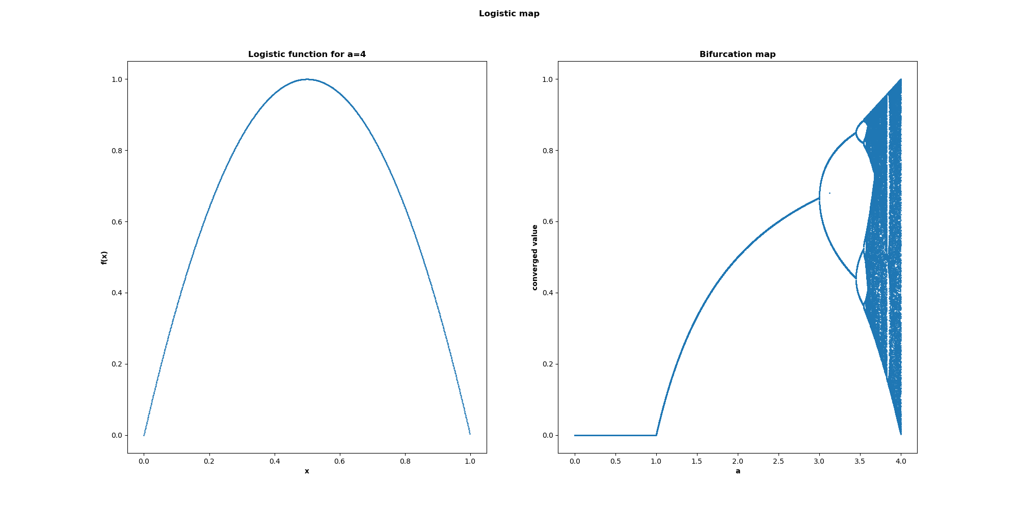
Analyzing the bifurcation map, we see a few distinct regions:

• For 0<=a<=1, the function is non-chaotic, always going to zero.
• For 1<=a<=3, the function is non-chaotic, always going to a single fixed point.
• For 3<=a<3.4, the function is non-chaotic, but bounces between 2 values instead of a single fixed point.
• For 3.4<=a<=3.57, the function is non-chaotic, but bounces around a few fixed values.
• For 3.57<=a<=4, the function is chaotic, never reaching a single fixed point.

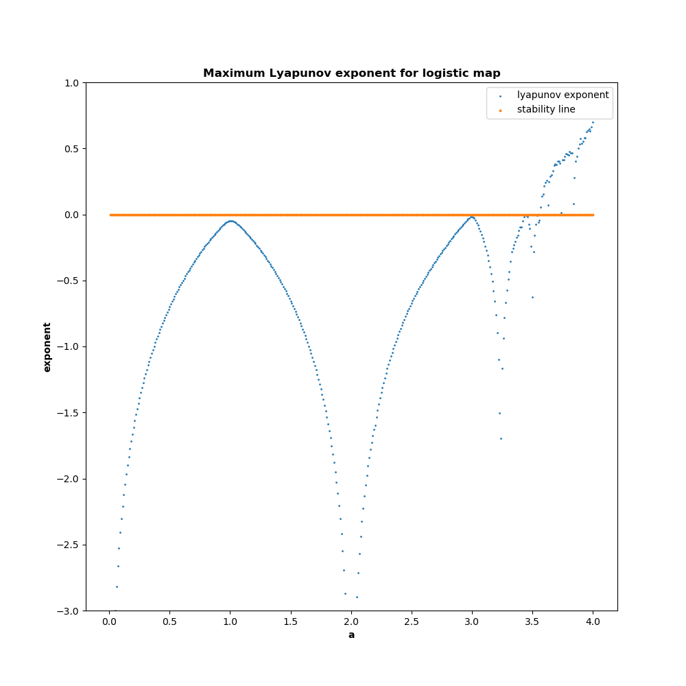
This pattern of multiple fixed points transitioning to chaotic behavior is common to many chaotic systems, called period doubling. We can also plot the Lyapunov exponent for each of the different values of A, yielding the plot below. This confirms that for the region 3.57<=a<=4, the logistic map displays chaotic behavior.

Chaotic lattices

At this point, we have examined the logistic map and verified its chaotic behavior. However, we still need a framework for harnessing the chaotic behavior to perform computations. One proposal put forth by Ditto and Sinha utilizes the following algorithm to create an analog logic gate:

• Every input gate has two input voltages, A and B
• Use the logistic map as the function f, with a=4
• Select an initial value (x0) and a critical value (xc), depending on the gate to be emulated
• Compute the input to the chaotic gate as accumulator = x0 + A + B
• Compute the output of the chaotic gate as chaotic = f(accumulator)
• Threshold the output using x_c such that output=max(chaotic-x_c, 0)

As part of the design process, these two values x0 and xc are selected for each logical gate to be emulated such that the outputs are either 0 or a common value d. By adding this constraint on the output value, these chaotic gates can be cascaded together, feeding the output of one gate into another like a traditional logic circuit. We can do a simple parameter search to find a few pairs of threshold and initial values that satisfy these constraints, with delta = 0.25:

| ---- | ----- | ------ |
| Gate | X0    | Xc     |
| ---- | ----- | ------ |
| AND  | 0     | 0.75   |
| ---- | ----- | ------ |
| OR   | 0.125 | 0.6875 |
| ---- | ----- | ------ |
| XOR  | 0.25  | 0.75   |
| ---- | ----- | ------ |

As an example, consider the XOR gate. This gate’s output should be nonzero if the inputs are different. Crunching the numbers with x0=YYY and xc=ZZZ, we have

• A=0, B=0: accumulator = 0, chaotic = 0, output = 0
• A=1, B=0: accumulator = 0.25, chaotic = 0.75, output = 0
• A=0, B=1: accumulator = 0.25, chaotic = 0.75, output = 0
• A=1, B=1: accumulator = 0.5, chaotic = 1, output = 0.25

We can see here that an digital output of 1 corresponds to an analog voltage of xxx, and a digital output of 0 corresponds to an analog voltage of 0. If you perform the same exercise for each of the other gate values, you will see that for each gate, the digital output of 1 corresponds to the same voltage. This is critical; if it were not so, then gates could not be composed without additional processing circuitry.

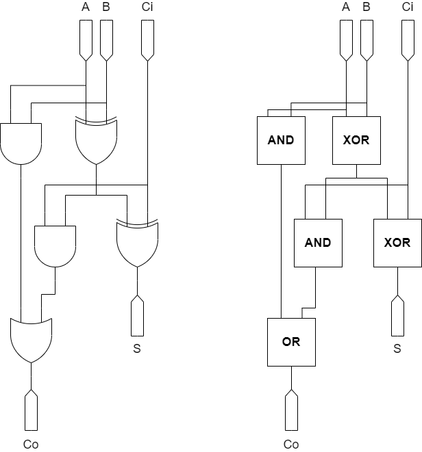
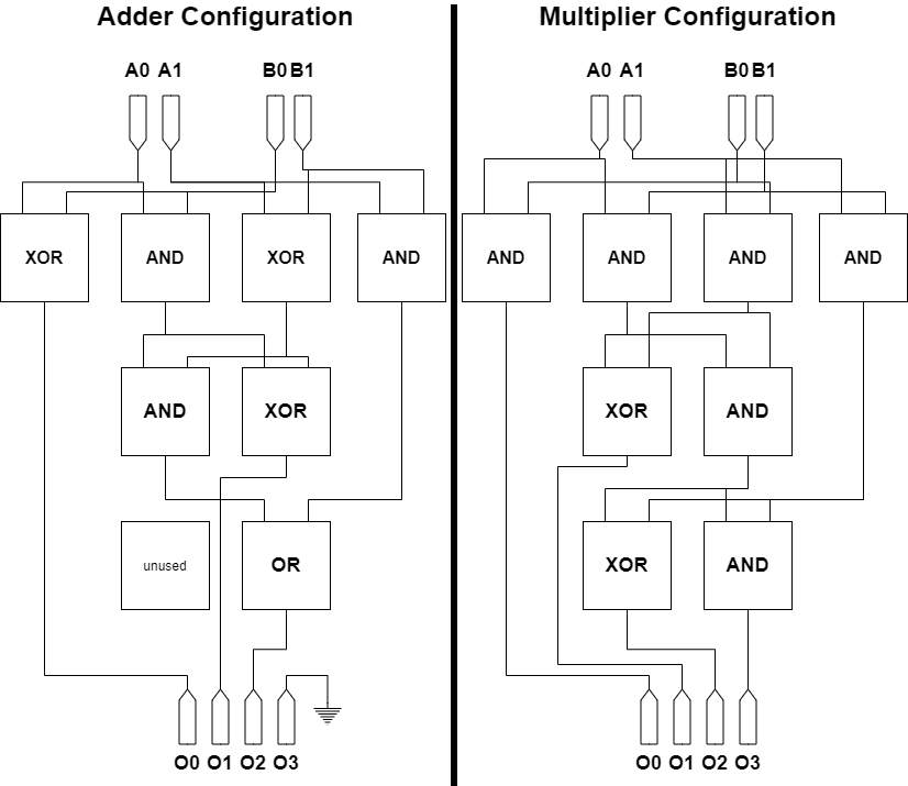
This concept of interconnected chaotic gates is called a “chaotic lattice”. This is the chaotic equivalent of a logical circuit. Shown below are two implementations of a full adder. On the left, traditional logic gates are used, where on the right, chaotic gates are used. The circuits are nearly identical, but with the chaotic computer, the gates could be theoretically re-used for a different function if the adder is not currently in use.

Adaptation to digital logic

While the framework described above is impressive, one implementation issue is the use of analog voltages for computation. Analog circuitry is more fragile and more difficult to miniaturize than digital circuitry. In addition, in order to interface with other digital logic, the signals would need to be converted to analog and back, which is expensive and time consuming. We can try to compute the logistic function digitally, but this runs into another problem - computational expense. To compute the logistic function, we need two multiplies and a subtract. While this might not sound excessive, this is many times larger than a single logical gate. In addition, many bits of precision must be kept in order to compute the correct result, further increasing the amount of resources required. Finally, there are limited gates available - for the full flexability of the implementation, we’d like to be able to define negation gates like NAND, NOR, and XNOR, which cannot be represented in a small number of bits with the logistic function.

Fortunately, there is a version of this function that is more palatable to digital computation. Introduce the tent map function:

f(x) = a * min(x, 1-x) 

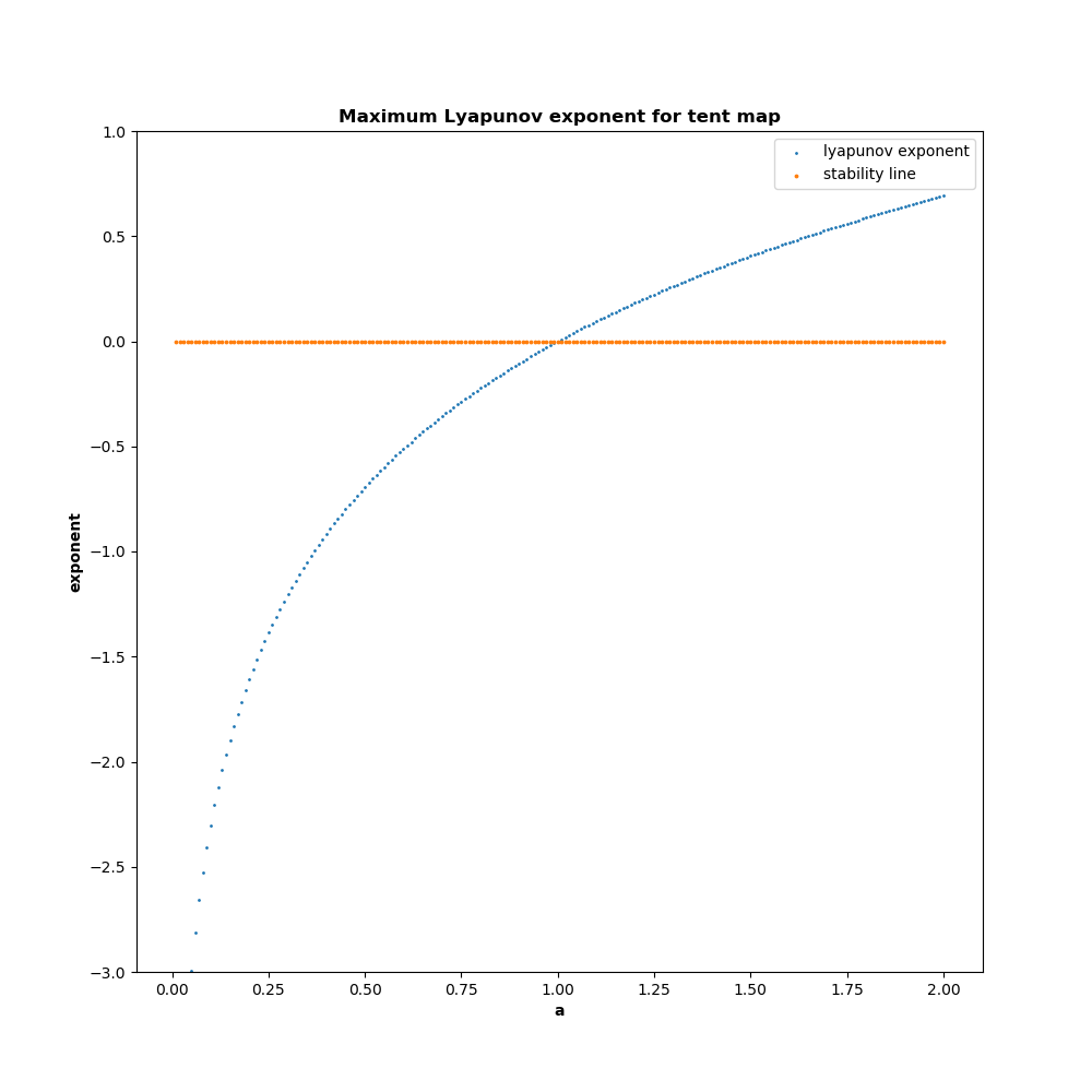
By using the transformation x' = (2 * arcsin(sqrt(x)) / pi), we find that the logistic function is homeomorphic to the tent map function with a = 2. Shown below at left is the tent map for a=2, and at right is the bifurcation map. The function shows the same period doubling behavior as the logistic map, and for a=2 appears to be chaotic.

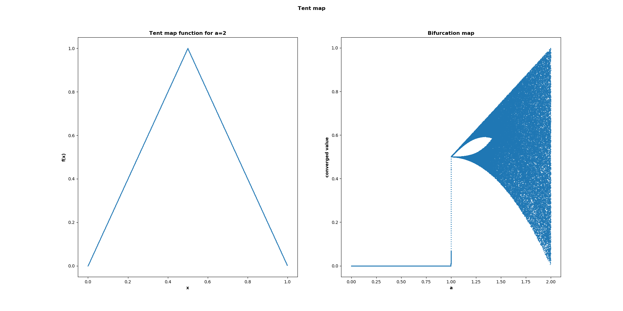
Computing the lyapunov exponent for various parameter values confirms that this function is indeed chaotic.

In addition to being computationally simpler than the logistic map, the chaotic parameters for these functions can all be represented with three bits, making it extremely cheap and space-efficient. Here’s an example set of chaotic parameters for a universal set of logical gates:

| ----- | ----- | ----- |
| Gate  | X0    | Xc    |
| ----- | ----- | ----- |
| AND   | 0     | 0.75  |
| ----- | ----- | ----- |
| OR    | 0.125 | 0.5   |
| ----- | ----- | ----- |
| XOR   | 0.25  | 0.75  |
| ----- | ----- | ----- |
| NAND  | 0.375 | 0.5   |
| ----- | ----- | ----- |
| NOR   | 0.5   | 0.75  |
| ----- | ----- | ----- |
| XNOR  | 0.75  | 0.25  |
| ----- | ----- | ----- |

In addition, via experimentation, it is possible to find an equivalent set of parameters with a=1, allowing us to save the multiplication.

| ----- | ----- | ----- |
| Gate  | X0    | Xc    |
| ----- | ----- | ----- |
| AND   | 0     | 0.25  |
| ----- | ----- | ----- |
| OR    | 0.125 | 0.125 |
| ----- | ----- | ----- |
| XOR   | 0.25  | 0.25  |
| ----- | ----- | ----- |
| NAND  | 0.375 | 0.125 |
| ----- | ----- | ----- |
| NOR   | 0.5   | 0.25  |
| ----- | ----- | ----- |
| XNOR  | 0.75  | 0.75  |
| ----- | ----- | ----- |

Armed with these optimizations, we are ready to implement the chaotic lattices on an FPGA and see how well they work in practice.

Experimentation

In order to see how well these universal logic gates work in practice, we implement them on a DE0-Nano development board. This board an Alterra Cyclone IV FPGA, which can be programmed with VHDL. The application we implement is a 2-bit adder which can be morphed into a 2-bit multiplier via a toggle switch. Each of the 2-bit inputs can be toggled via a toggle switch, and the output can be seen on the string of LEDs present on the device. The chaotic lattices for the 2-bit adder and multipliers can be seen below:

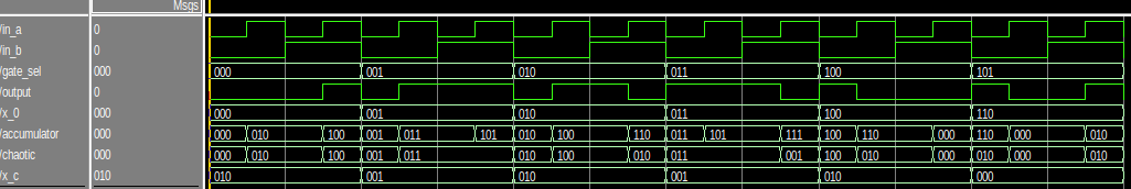
We create 2 implementations of the universal logic element, one using the naive approach and one using the chaotic computation approach. Before uploading the design to hardware, we design a simulation test bench to verify functionality. The results of the simulations with the chaotic elements can be seen below:

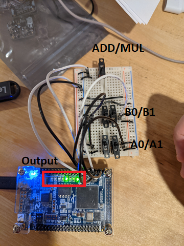
Finally, here is a picture of the experimental setup, with each of the inputs labeled. Also included is a short video of the operation of the device.

Discussion

One of the first approaches one may take when attempting to compute the lyapunov exponent is to collect data and treat it as a curve fitting exercise. That is, compute the trajectories for two points separated by an infinitesimal amount, take the difference, and fit an exponential curve to the difference. While this approach is theoretically valid, it hits a practical problem - the exponential functions overrun the limited domain of the output variable too quickly. For the logistic map, depending on the parameter there may be as few as 5 data points before the difference vector is aliased into oblivion. This makes curve-fitting error prone, as there are too few points to accurately compute the exponent.

Fortunately, there is a numeric trick. First, we can use basic algebra to rearrange the equation to isolate the exponent:

lambda = (1/t) ln(|dZ(t)|/|dZ_0|)

Next, we make the following assumptions:

• If the system is chaotic, the chaotic factor will be the dominant element present after a long time. This is because the chaotic effect grows exponentially, while non-chaotic effects are usually bounded by smaller elements.
• We are interested in starting the points as close together as possible.

For this estimation, we can add the following limit statements:

lambda = lim(t => inf) lim(dZ_0 => 0) (1/t) ln(|dZ(t)|/|dZ_0|)

Because we have a discrete system, we can make the following approximations:

• Replace the dummy variable t with n.
• Linearize the system using euler’s method
• Realize that dZ(t) = f(t+dZ(0)) - f(t).

From the last point, we can use the definition of the derivative to replace the term inside the logarithm with f'(x), yielding the following numerical expression:

lambda = lim(n=>inf) (1/n) sum(i=0..n-1)(log(|f'(x_i)|))

In addition to being faster to compute, this result is much more numerically stable. We can see that for most of the values of a, the two algorithms give approximately the same result, but the method with these numeric optimizations is much smoother.

Sharp readers might relize that there is another chaotic function which we may have chosen to use, the Dyadic map. This transform, sometimes called the “sawtooth transform” for the shape of the graph, has the form f(x) = (2x) % 1. This expression is even cheaper to compute than the tent map, however, it does come with a significant drawback. It turns out that there are no critical pairs for X0, Xc, and delta that satisfy the requirements for the universal gates with less than 12 bits. This means that while the computation engine may be simpler, more bits would have to be used to store the information required to properly initialize and threshold the output - ultimately making it a worse choice than the tent map. This function is still interesting due to its simplicity, but in order to effectively use it a new computational framework would have to be developed.

When compiling the circuits for hardware, the QuartusII compiler will compute resource usage in terms of LUTs, or LookUp Tables. These are the fundamental unit of space when compiling for FPGAs. Although they are not directly comparable to transistor count, they provide a rough approximation - a design that would use more transistors will generally use a large number of LUTs. In our design, both the chaotic and naive implementations take the same number of LUTs - 8 - meaning that despite the higher complexity, it’s likely that the designs would use the same order of magnitude of resources.

However, there are still some large problems to solve before this technology becomes production viable. First, there is the problem of gate latency. When inspecting the code for the universal gates, we see that there is a long sequential pipeline that needs to execute for each computation. When synthesized into hardware, this translates into a longer latency between an input signal change and an output signal change. Practically, this would force clock rates to decrease, dramatically decreasing the performance of the hardware.

In addition, there is the problem of routing. Consider the input layer of the chaotic lattices for the adder and multiplier. For the adder, these gates accepted A[1], B[1] and A[0], B[0] for the inputs A and B. However, for the multiplier, they operated also on A[1], B[0] and A[0], B[1]. For this toy implementation, we could use a simple CASE block to swap between them, but for more complex designs, there would need to be some form of logic that could “route” the inputs and outputs of the gates to each other at runtime on the fly. This is not a simple task, especially when we consider that these routings should not be static but dynamically reconfigurable to deal with hardware failures. The lack of this routing layer is a major roadblock which prevents this from replacing current technologies.

Finally, although the field is called “chaotic computing”, it doesn’t appear as if chaos is strictly necessary. When looking at the tent map, we were able to find an implementation for gates when a=1. As evidenced by the lypanov exponent computation and by inspecting the bifurcation map, this function is not chaotic for this parameter value. Instead, it appears as if all we really need is a nonlinearity. We can get away with this because we are not depending on the long-term behavior of the function - we are merely running it for a single iteration.

So, where does this leave chaotic computing? In its current state, chaotic computing might be a good fit when the following conditions hold:

• There is a desire for “morphable hardware”
• The functions that need to be morphed between have a similar structure
• High performance is not a strict requirement

As of today these restrictions leave us with few practical applications, but as better basis functions are found and better schemes for routing are discovered, these downsides may become less severe.

Summary

In this post, we examined the scheme proposed by Ditto and Sinha for utilizing chaotic functions as a universal basis for reconfigurable hardware. We examined the initial proposal and made some optimizations that allowed the function to run efficiently on digital hardware. As a proof-of-concept, we built a morphable computer that could switch between multiplication and addition while re-using the same hardware gates. Finally, we made some observations on the current state of chaos computing as a competitor for current fixed-gate technologies, as well as speculated on the future of this technology.

Downloads

The code that has been used to generate all plots, artifacts, and analysis can be downloaded from Github here.