Introduction

Image processing is one of the most popular applications of machine learning today. Many different algorithms have been proposed to attempt to extract meaning from images, with a wide variety of potential applications. Currently, most state-of-the-art approaches tend to use deep learning, which attempts to build an artificial model of the human brain. Once architected, these deep networks are trained on a vast amount of data, learning the proper representations to separate the signal from the noise. While a properly trained deep network can yield impressively accurate predictions, there are a few drawbacks to using this type of model in a production setting:

• Computational cost: Neural networks are computationally expensive to run, as running an inference typically involves multiplying many large matrices together. In addition, training a network is expensive, oftentimes requiring large quantities of special-purpose hardware such as GPUs.
• Data Requirement: Training a deep neural network requires a vast amount of data to converge. With too little data, neural networks can risk overfitting, which yields disastrous results.
• Restrictions on Loss: In order for neural network training to work, loss functions are required to be fully differentiable. This means that it can be difficult for the network to learn functions that have discontinuities. An example of this would be if a network wanted to include performance as a loss parameter. Performance typically depends on the number of weights added, which can only be added in discrete increments, making the loss function discontinuous.
• Interpretability: The output of a deep neural network is a series of “weights”, or a dense chunk of numbers. It is difficult to tell what the network has learned, and why it makes the inferences that it does.

There is an alternative to deep learning, which is Cartesian Genetic Programming. Cartesian Genetic Programming (CGP) is an evolutionary algorithm which attempts to model the learning problem via the principal of natural selection. In this algorithm, a series of candidate solutions are generated, then evaluated via a “fitness function.” Candidates that receive a higher score will be used to generate the next generation of candidates, and those that have a lower score will be discarded. Over time, the system will converge on an optimal solution, which will then be used for inference. On first glance, CGP seems to address many of the concerns with deep neural networks:

• Computational Cost: CGPs use an embarrassingly parallel training procedure, and can be quickly trained on the CPU. So it is trivial to scale out a CGP training algorithm to many nodes.
• Data Requirement: CGPs tend to work on much less data than deep neural networks. In fact, some recent papers (see below) have shown very good results with ~10 training samples. This is a huge savings compared to the hundreds of thousands of examples needed for a deep neural network.
• Restrictions on Loss: CGPs can accept an arbitrary loss function, which makes it trivial to combine multiple loss metrics into a single function.
• Interpretability: While deep networks generate weight matrices, the output of CGPs are computer code (e.g. a c++ function). This makes it easy to see what the network is doing, as well as debug the different phases of the algorithm.

Recently, there have been a few papers have shown very good results applying CGP to image processing tasks. In this experiment, we will develop a framework for training CGP algorithms. The framework will be designed to be extensible, so that it can be rapidly applied to any problem. The framework will then be applied to three problems. First, a simple curve-fitting problem. Next, a simple semantic segmentation problem in which a playing card will be extracted from an image. Finally, the framework will be applied to a more complex problem, that of picking out buildings from a satellite images. Along the way, observations will be made to see to what extent CGP offers a benefit over deep neural networks, and develop an intuition regarding when they should be used.

Theory

Evolutionary algorithms are a class of algorithms that attempt to learn by imitating natural selection. These algorithms typically begin with a set of randomly generated candidate solutions, divided up into a set of “islands.” For each iteration of the algorithm, two steps are performed, selection and generation. For the selection phase, each candidate is evaluated by some fitness function. These fitness functions are analogous to loss functions in deep neural network training, in that they give a scalar score to each candidate, allowing them to be ranked. After evaluation, the few best performing solutions are kept for the next generation, and the remainder are discarded. Once selection has been performed, new solutions are generated from the best candidates from the previous generation. This can be done in a variety of methods, the most common of which are combination and mutation. With combination, two candidates are mashed together in some manner to generate a new solution. With mutation, a small random modification is made to the generated solution. Each island performs the optimization separately, and occasionally the best solutions from each islands are introduced to the other islands. Over time, the only solutions that will remain are those that have a high fitness, leading to a good solution. A basic pseudo-code implementation for an evolutionary algorithm might look like this:

def island_iteration():
    candidates_with_scores = []
    for candidate in island_candidates:
        score = fitness_function(candidate)
        candidates_with_scores.append((candidate, score))

    sort(candidates_with_scores, score, order=descending)
    
    island_candidates = []
    for i in range(0, num_candidates_to_keep), 1):
        island_candidates.append(candidates_with_scores[i][0])

    while (len(island_candidates) < island_capacity):
        p1 = select_random_parent(island_candidates[:num_candidates_to_keep])
        p2 = select_random_parent(island_candidates[:num_candidates_to_keep])
        new_candidate = crossover(p1, p2)
        new_candidate = mutate(new_candidate)
        island_candidates.append(new_candidate)

def evolve():
    islands = randomly_initialize_islands()
    for i in range(0, num_iterations, 1):
        for island in islands:
            island_iteration()
        
        if ((i % island_sync_period) == 0):
            candidate = find_most_fit_candidate(islands)
            introduce_best_candidate(islands)

    best_candidate = find_most_fit_candidate(islands)
    return best_candidate

Within this class of algorithms, there are a few different subclasses which primarily differ in the manner in which the candidates are represented. The first example of an evolutionary algorithm was the genetic algorithm, which was first proposed in the 1950s by Alan Turing. In this formulation of the problem, each candidate is a “bit vector”, or a string of 1s and 0s of a fixed length. Crossover can be accomplished by taking two candidate solutions and selecting half of the bits from each. Mutation can be accomplished by randomly flipping one or more of the bits. On each iteration, the bit vectors would each be passed to the fitness function, which would then determine the quality of each of the solutions.

A classic example of a problem that can be solved with a genetic algorithm is the knapsack problem. In this problem, there are a set of objects, each with a weight and a value. There is also a knapsack which can only hold a finite amount of weight. The goal is to figure out the set of items that can be placed into the knapsack which achieves the maximum value without going over the knapsack’s weight. For this algorithm, the optimal algorithm runs in exponential time, so it can only be exactly solved for a very small number of items. To use a genetic algorithm for this problem, one possible formulation would be treating each candidate as a bit vector whose length is the number of items. A 1 in position n would represent that the n-th item is taken, while a 0 would represent that the item is not. The fitness function would sum the values of the weights and the items, returning the sum of the values if the weight is less than the knapsack’s weight, and 0 otherwise. Using this procedure, one can achieve a close-to-optimal solution in a small fraction of the time needed for the classical algorithm to run.

While genetic algorithms are convenient for problems involving discrete optimization, they require the designer to come up with a representation of their problem that can capture all of the semantics within a bit string. This can be impossible for more complex problems, like image processing. In addition to needing an absurdly large number of bits to represent the images, combination and mutation can only be performed at a very specific point in order to still yield a valid algorithm. So while useful for some problems, the genetic algorithm cannot be used for everything.

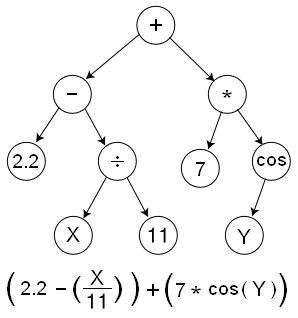
An alternative to the genetic algorithm is the genetic program. Rather than use a bit string to represent the candidate, genetic programs represent an actual computer program. In their initial implementation, each program was represented as an abstract syntax tree, where each node was a function chosen from a pre-defined set of inputs, called “basis functions”. For example, if the application was curve fitting, the basis functions might be simple mathematical operations such as add, subtract, exponentiate, divide, etc. The connections between nodes would represent the flow of data, as the basis functions get combined into a complex series of nodes. Crossover could be defined by carefully swapping parts of two trees, and mutation could be performed by swapping out one of the basis functions within the tree with another one. A visual example of a genetic program can be seen below:

While this representation is intuitive, it comes with its fair share of problems. First, tree data structures are tricky to program, especially in high-performance languages with manual memory management such as C++. Second, defining the crossover and mutation operators are difficult, as one needs to be careful to validate that the output program is still valid. For example, one cannot replace an add node with an exponentiation node, because add takes two arguments, and exp takes 1. Finally, trees can suffer from a problem called “bloat,” in which trees grow without bound over time. This happens because in the simplest formulation, there is no restriction on the size of the tree, so the algorithm will continue to add more and more nodes to the tree in order to attempt to improve the fitness. This can lead to overfitting, as well as algorithms that are different to understand and interpret.

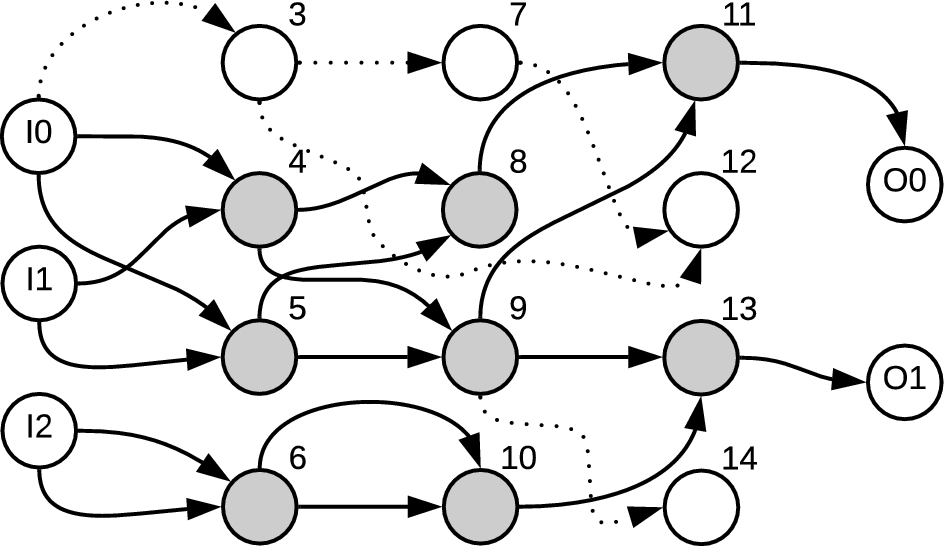
There is another representation which elegantly solves these problems, called the Cartesian Genetic Program (CGP). In this representation, the same basis function is used, but instead of representing it as a tree of nodes, a fixed 2-d grid is used. This 2-d grid is called a “genotype.” A visual representation of the genotype is shown below. Here, the leftmost nodes are the inputs, the rightmost nodes are the outputs, and the gray nodes in the center are the genes. Each gene is associated with a basis function, as well as a set of parameters for the particular basis function. For example, one of the genes might be “add”, and another might be “Output the constant value 2.” In the simplest formulation, each gene can have a connection to any gene in a column further to the left. This rule avoids cyclic dependencies. Once the nodes are connected, the output of the algorithm is selected to be a random node of the grid. This means that not all genes contribute to the output. The genes which do contribute to the output are called “active genes,” and a genotype stripped of all inactive genes is called a “phenotype.” This means that multiple different candidates can have different values, but represent the same physical algorithm because the only differences are in inactive genes. In other words, one phenotype can be represented by multiple different genotypes, but one genotype always yields one phenotype.

Typically, with CGP, crossover is not performed during the generation phase. Instead, new candidates are generated using only mutation. For each iteration, genes are randomly mutated by either randomly swapping their basis function, their parameters, or their input connections. There are a variety of ways to determine how many genes to mutate on each iteration, but an elegant solution is to continue randomly choosing genes to mutate until an active gene changes. The intuition is that if a mutation is made to an inactive gene, then the phenotype is the same, yielding the same fitness function. Therefore, there is no reason to reevaluate it.

Representing the problem in this manner is much easier to program because the grids are of fixed size. In addition, this representation elegantly solves the bloat problem, because the grid of a fixed size. For a much more in-depth introduction to how CGP works, consult this excellent reference from Springer. For a broader overview of genetic programming in general, consult this excellent survey paper from the KSII Transactions on Internet and Information Systems conference.

Framework

Unfortunately, there don’t appear to be many frameworks available for writing CGPs. This is likely because genetic programs are hard to write in a generic method, as much of the power comes from carefully chosing the basis functions. Choosing good basis functions generally requires domain knowledge, so it’s hard to write a generic framework like one can for deep learning. To run these experiments, a CGP training and evaluation framework was created. This framework is designed to be extensible, so that custom basis functions can be implemented via subclassing. To apply the problem to a different domain, one would simply need to implement the basis functions using the provided class templates. Once implemented, the user can specify a training configuration (e.g. which basis functions to use, number of genes in the grid, number of iterations, etc) via a JSON configuration file. The framework supports the following quality-of-life features:

• Extensibility: The framework has many extension points, making it easy to customize to a particular problem. The code is also open-sourced with a GPL license, so it can be modified if the need arises.
• High performance: The framework is implemented in C++. It is designed for high throughput, capable of using all available cores on the system. In addition, memory mapping is used to take advantage of the available system RAM, avoiding the need for expensive I/O during training.
• Periodic checkpointing: During the training process, checkpoints are periodically made. This can allow one to monitor the training process and restore if there is an error.
• Solution visualization: Once trained, a graphviz file can be generated, which shows the different nodes and their connections. For image problems, this can be used to create a visual flow diagram of the solution, aiding debugging and interpretability of the algorithm.
• Code generation: Once trained, a c++ file can be generated which implements the genetic algorithm. This C++ file can then be included in another application and used for inference. Apart from OpenCV, the code does not have any dependencies on the training library, so it is easy to integrate into any other project.

For more information about the framework, consult the readme on the github page.

Application: Curve Fitting

The first test for the CGP framework will be a simple curve fitting application. For this application, a data set was generated using the following equation:

y = (2*sin(3*x)) - (0.4 * x) + 1, x ∈ [-10, 10]

The basis functions implemented were simple arithmetic functions:

• Add: accepted two inputs, A and B. Outputs A+B.
• Subtract: accepted two inputs, A and B. Outputs A-B.
• Multiply: accepts two inputs, A and B. Outputs A*B.
• **Divide Protected: accepts two inputs, A and B. if B is zero, outputs 1, otherwise outputs A/B.
• Sin/Cos: Accepts one input, A. Computes sin(A) or cos(a).
• Constant: Accepts zero inputs. Outputs a constant value.

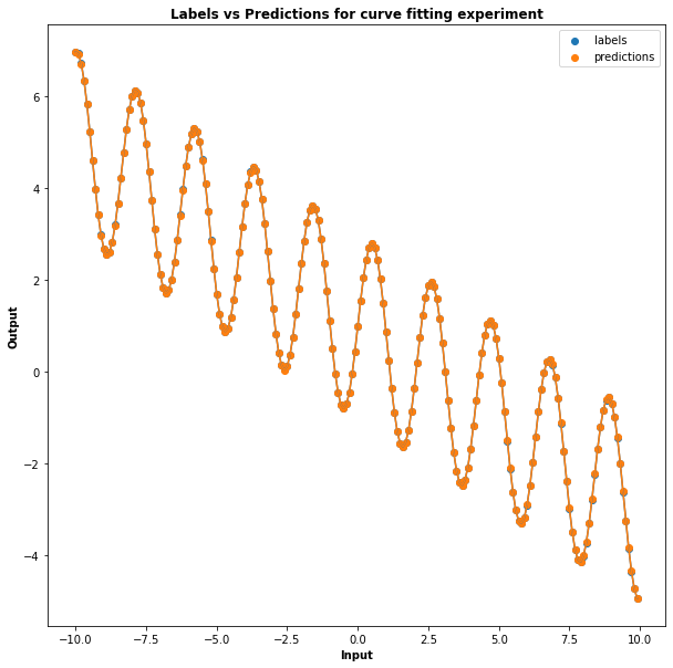
The implementation for these basis functions can be found here. Using these seven basis functions, a CGP model was trained until convergence. After only a few hundred epochs, the solution converged on an almost perfect fit. The image below shows a plot of the predictions and the labels, which agree almost perfectly.

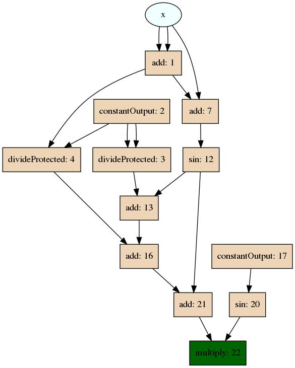
A visualization of the learned solution can be seen below. By examining the genes that are included in the graph, we can see that it corresponds to the equation that was used to generate the curve, showing that the model has indeed learned the proper solution. For the curious, the full experiment configuration, which includes all parameters used to reproduce this result, can be found here.

When examining the basis functions, one might wonder if all of them are strictly necessary. For example, subtractions can be achieved using an add gene after negating one of the arguments. One might ask is it better to have fewer, simpler basis functions or a larger number of more complex ones. Fortunately, this is easy to test. For this test, two sets of CGPs were trained on the same curve fitting data set. One set used the full set of 7 basis functions, as shown above. The other set used a subset of these basis functions - add, constant value, multiply, and sin. Each configuration was trained 5 times until convergence, only changing the random number generator seed between runs. In all cases, the CGP managed to generate a nearly perfect (e.g. L1 error of <.000001) fit to the curve. The major difference, however, was in the training time. The plot below shows fitness as a function of time, in which 0 fitness is equivalent to a perfect fit.

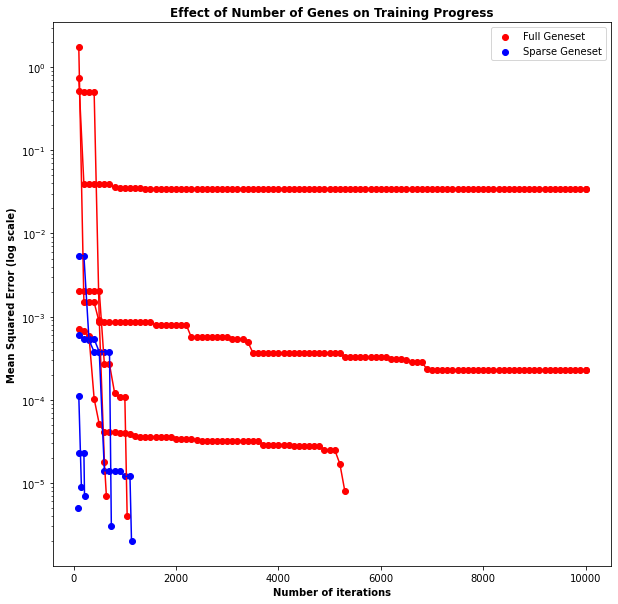
The algorithms trained using fewer basis functions took drastically less time to converge than those with more basis functions. This makes sense - increasing the number of basis functions dramatically increases the size of the search space. While this may be necessary for more complex problems, in this case it did not provide any benefit. This result shows how important it is to carefully select the proper basis function for the application. Too few basis functions, and the model will be incapable of learning the relationship between input and output. Too many basis functions, and the model will fail to find the optimal solution, as the search space will have grown extremely large.

Application: Target Detection

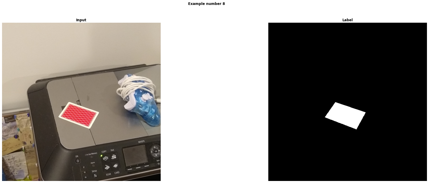
Next, we turn our attention to how to use CGP for image processing. To test the capabilities of the algorithm on this type of problem, we will attempt to perform a simple version of template matching. A data set of 9 images is generated by placing a red playing card in a few natural scenes. The images are then annotated with bounding box information, and pixel-wise labels are generated where each pixel is 255 if the pixel is within the card’s bounding box, and 0 otherwise. An example image, along with the generated label, is shown in the image below.

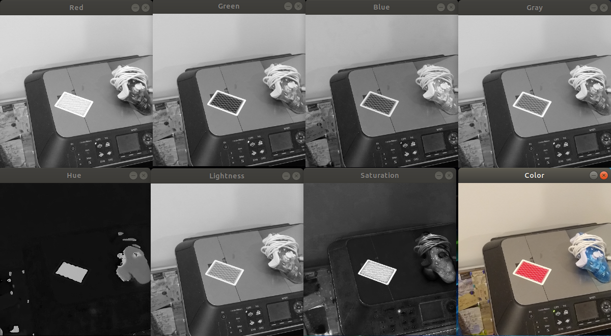
For this, we follow the approach outlined in the springer paper which introduced the algorithm. The first difference between this application and the curve fitting is the representation of the input data set. Instead of a single input, there will be 7 inputs, each a 2-d array of unsigned chars representing a portion of the image data. The first three inputs are the Red, Green, and Blue channels, respectively. After transforming the image into Hue-Saturation-Luminance (HSL) space, these three channels represent the next three inputs. The last channel is generated from the grayscale pixels of the image. The image below shows the sample image from the card data set along with each of these different generated inputs.

We then implement each of the 40 basis functions described in the paper. The full list and implementation of basis functions can be found here, but the descriptions generally fall into a few categories:

• Pixelwise arithmetic operations: Operations like pixelwise add, pixelwise exponentiate, and pixelwise square root.
• Blurring operations: Operations like Gaussian blurring or bilateral smoothing.
• Thresholding operations: Operations like binary thresholding.
• Edge Detection: Operations like canny, laplace, or sobel.
• Texture detection: Operations like gabor filtering.
• Morphological operations: Operations like eroding or dilating.
• Normalization operations: Operations that tended to rescale the pixels to their full range.
• Shifting operators: Operators that shift the image in a certain direction (e.g. left 2 pixels).

Many basis functions exist in both a local version and a global version. For example, the normalize operator. This operator computes the minimum and maximum pixels, and rescales the pixels linearly such that the new minimum pixel value is 0 and the new maximum is 255. The global version considers the entire image, while the local version considers only a small neighborhood around each point. Each of these genes leveraged OpenCV in order to improve performance.

For the fitness function, using the obvious choices of L1 or L2 loss did not yield good results. This is because the data set is quite unbalanced - there are many more non-card pixels than there are card pixels, so the model gets stuck in a local minimum that just outputs all zeros. Instead, we use the Matthew’s correlation coefficient (MCC), which provides a more unbiased view of the model’s performance. For MCC, 1 or -1 represents perfect predictions (-1 meaning that the classes are reversed), and 0 represents that the output labels are no better than random chance. Because our framework views lower values of fitness as preferable, we use the following fitness function:

fitness = 1.0 - |mcc(predictions, labels)|

After training for a few hundred epochs, we are again able to successfully genearate a CGP which can solve the task. Shown below is one of the images reserved for testing, along with the true and predicted labels. For the curious, the full configuration used is here.

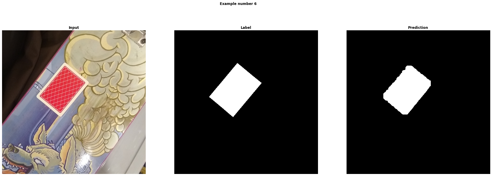
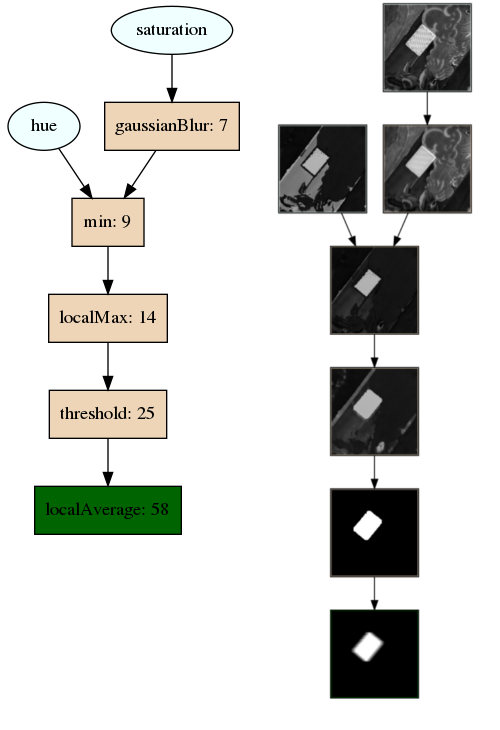
While not perfect, the algorithm performs suprisingly well given that there are only 9 input images on which to train. To train an equivalent deep network from scratch, a minimum of thousands of images would be needed! A visualization of the trained algorithm can be seen below. The graph on the left shows the operations that are performed to generate the outputs from the inputs. The graph on the right shows the images at each step of the prediction.

It appears as if the CGP can accurately solve this task, but one may wonder if it can solve it while also optimizing performance. Some of the basis functions above, such as pixel-wise addition, are extremely cheap to compute. Other, such as bilateral filtering, are extremely expensive. Ideally, we’d like our algorithm to use the simpler options if it doesn’t make a huge difference in performance. One of the ways we can do this is by creating a multi-objective loss, which includes terms for both correctness as well as runtime performance. For correctness, the MCC can be used, like before. To get a sense of how to incorporate runtime performance, we first run each basis function a few hundred times and compute the mean runtime for different parameter values. This gives us a distribution like below:

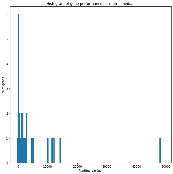
Some of these functions, such as bilateral filtering, depend heavily on the parameters used (in this case, the pixel window, “d”). Armed with this data, we can compute an estimated runtime cost for each operator. Assuming the time it takes to pass data between basis functions is negligible, we can then estimate the runtime cost of the algorithm by summing the runtimes of each active basis function. From there, we can define the full multi-objective loss:

loss = (1.0 - |mcc(predictions, labels)|) + (λ*runtime(phenotype))

Where λ is a constant used to balance runtime performance and correctness.

To test this multi-objective loss, we train CGPs on the card detection data set using different values of lambda. Each training task was performed 3 times, and the average results are shown in the plots below.

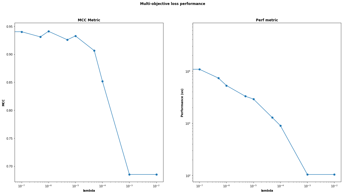
Here, we can see that as we increase lambda, the runtime performance gradually decreases until it hits a wall around λ = 0.001. Accuracy doesn’t change much until λ = 0.0001, with a significant drop-off past that point. Manually inspecting the modules generated when λ = 0.001, we see that the generated models generally have a single gene, which means that runtime performance was prioritized too highly. For this problem, using λ = 0.0001 appears to give the best of both worlds - a more performant final algorithm, while still maintaining a reasonable level of correctness.

Application: Building Detection

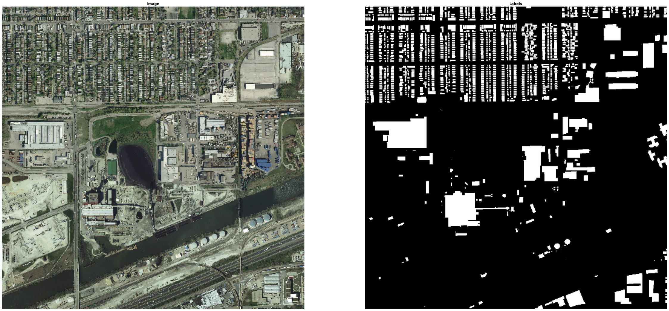
For a final application, we examine a more difficult image processing problem - semantic segmentation on satellite imagery. For this problem, we use the Inria Aerial Image Labeling Dataset data set, which contains arial images captured over N different cities. In addition to the high-resolution images, pixel-wise labels are generated that are 255 if the pixel resides within a building, and 0 otherwise. A few samples from this data set, along with their associated labels, are shown below.

This is a much more difficult problem than the card detection problem posed earlier, for a few reasons. First, the definition of a “building” is much more fluid than that of a playing card. Buildings do not have consistent shapes or color schemes. Even if perfect polygon detection could be performed, semantic information would be needed to determine which of these shapes are buildings and which are not (e.g. pools, cars, etc). In addition, the buildings are not always fully visible, e.g. when they are occluded by trees.

To generate the data set, 2 500x500 regions of interest were taken from each of the input images and preprocessed into their channels as described in the card tracking experiment. The same training parameters were used for the card experiment, although no performance loss was introduced (i.e. λ = 0). Two configurations were used, one with 100 genes in the grid, and one with 1000 genes.

In both cases, the models failed to generate high quality predictions. While there were a few initial signs of life, overall the predictions were of very poor quality. Shown below is the output of the most successful training. Notice how the blobs for the predictions are in the right place, but the shapes are not correct.

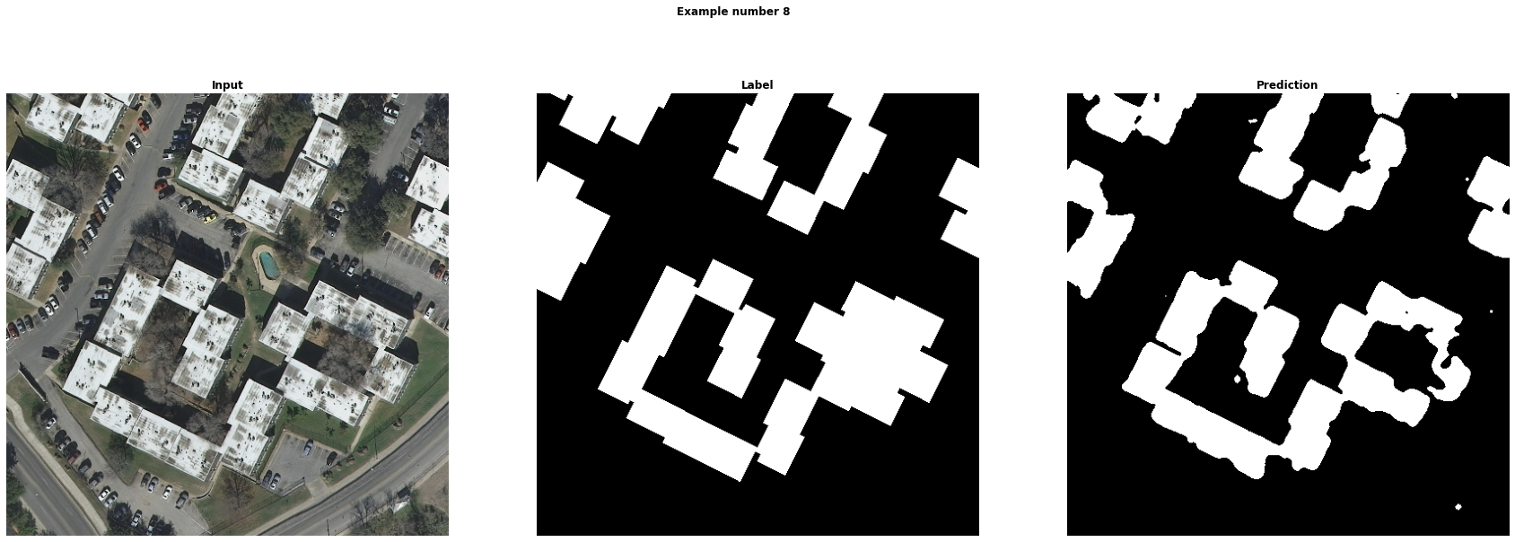
Increasing the number of genes did not have any noticeable impact on the quality of the predictions; rather, it only increased the runtime of the algorithm.

Discussion

When looking back at the two image tasks, the major difference between them is that the building detection problem required the use of higher-level semantic information to be successful, while the card detection one largely did not. Looking at a small region of the image, it is relatively easy to tell if it is a card - if it’s a large block of red, then it is a card. For buildings, this is much more difficult. Deep networks, which are the standard approach to semantic segmentation problems, typically solve this by using down/up sampling, such as with the U-net architecture. This is easy to do in deep learning, because when one predefines the architecture they can ensure that the shapes of the data tensors are such that data flows through the system in a logical manner. However, for CGP, this is much more difficult - instead of being able to freely interchange nodes like the algorithm requires, one needs to take care that only compatible inputs are connected. For example, one cannot do a pixel-wise addition of two tensors that are of different sizes. In order to incorporate higher-level semantic information, one would need to manually build a pyramid and train a separate CGP for each octave, then somehow recombine them. In addition to being much more computationally complex, propagating loss back through the different levels of the pyramid becomes difficult.

When viewing the outputs of the image processing experiments, it is interesting to see that the genes that show up in the best phenotypes generally contain very simple functions. The more complex functions, such as gabor filtering or morphological operations don’t appear to be used that often. This is odd because if hand-designing an algorithm, typically one would include a few of these algorithms in order to remove some of the noise present. For example, it’s typical to end the algorithm with a dilate/erode cycle to remove white “speckles” from the image. The generated functions are also complex and hard to understand, reducing the interpretability of the model. This is important because one of the top rationales for choosing the CGP is the model interpretability; if the output is too complex and interpretability is required, then another method should be chosen.

Given the above experiments, the CGP seems to be a good candidate for a learning algorithm when the following conditions hold:

• The problem has a very small amount of training data available.
• It is known that the solution can likely be expressed in terms of a small number of domain-specific basis functions, run in an unknown order with unknown parameters.
• The problem definition is fairly rigid, not requiring reasoning about ambiguous quantities.
• The acceptance criteria is composed of multiple objectives, some of which are not differentiable (e.g. performance).
• There is a way of evaluating the fit in an efficient and safe manner, as thousands of iterations will need to be performed for most problems.

There are many optimization problems that fit the bill. For example, curve fitting or task scheduling algorithms are well suited for CGPs. In these cases, we already know from experience the types of functions that would be useful, we just don’t know the optimal way to combine them or proper parameter values. However, there are many problems that are ill-suited for CGPs, such as perception problems. In this case, it is hard to choose a set of basis functions that can reasonably represent the solution. In that case, it is better to choose a different algorithm such as a deep net.

Summary

In this experiment, we built a framework for training Cartesian Genetic Programs. We apply this framework to three problems: a simple curve-fitting application, a simple perception problem, and a more complex perception problem. We observed the effects of choice of basis functions on the efficiency of the training process, as well as the use of multi-objective loss to balance conflicting objectives. After analyzing the results of the three experiments, we developed an intuition of the types of problems that CGPs would be useful for, as well as the types of problems in which they would be a poor choice. Choice of model type is one of the key decisions to make when attempting to solve a problem with machine learning, and realizing the strengths and weaknesses of each individual model type is critical to delivering a high-quality model.

Download Links

CGP Training Framework