Introduction

In previous experiments, we built a robust teleoperated robotic platform. While teleoperated robots are useful, autonomous robots are even more useful. In this project, the teleoperated robotic platform is given both hardware and software upgrades in order to allow it to compete in a simplified version of the Seattle Robotics Society RoboMagellan competition. This robot is capable of autonomously navigating in an a-priori unknown outdoor environment. The robot will be supplied with the general location of a target, which will be marked with an orange traffic cone. The goal of the robot will be to navigate from its starting location to the cone, avoiding all obstacles in its path.

Perception Stack

Sensors

One of the fundamental capabilities that the robot needs to complete this task is the ability to sense obstacles in its path. In addition, it needs to be able to detect the traffic cone marking the target location. A few different combinations of sensors were tried:

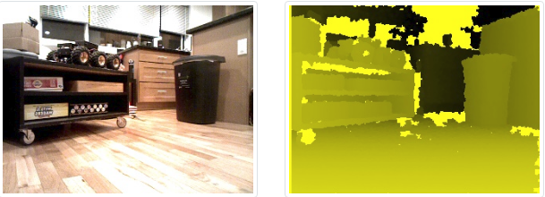
The first attempt was to utilize an Asus XTION depth sensor. This sensor is one of the less expensive 3-d depth sensors on the market. The output of this sensor comes in two parts: an RGB image and a depth image, which approximates depth to each pixel. The picture below shows a sample output. The left image is the RGB image returned from the sensor, while the right image is a visualization of the depth sensor output - closer points are brighter.

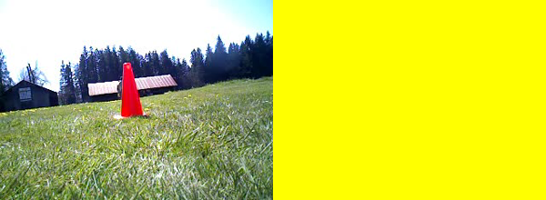
Unfortunately, this sensor performed extremely poorly in the sunlight. Because the sensor uses IR light to determine depth, even a moderate amount of sunlight causes the sensor’s output to become corrupted. Shown below is an example of this sensor taken in the bright sunlight - notice how the depth image is a single color of yellow.

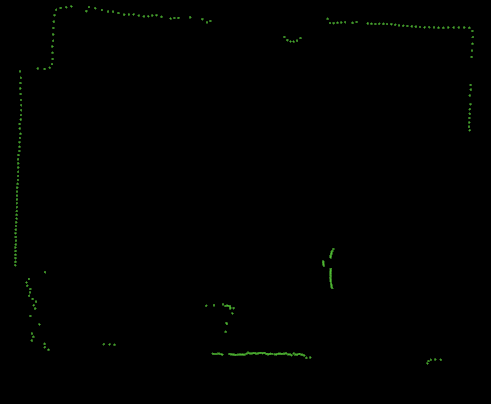
The next attempt was to use a RPLidar A3 sensor. This sensor is a time-of-flight LIDAR which is advertised to give millimeter-level accuracy in even harsh outdoor environments. The output of this sensor is a 2-d point cloud, or a “circle” of points. Shown below is a sample output of the sensor in an indoor environment.

Although the sensor was advertised as an “outdoor lidar”, it also performed extremely poorly in the sunlight. Even moderate amounts of sunlight caused the lidar to return corrupted readings. In addition, because the lidar was 2-d, it would not be able to detect obstacles that were below the scanline. For example, if there were a rock that were 8 inches high, the lidar would not be able to detect it. The combination of these issues made the lidar unsuitable for this robot.

After these two failures, a successful solution was found in the form of the ZED2 stereo camera. The ZED2 combines two high-definition cameras and an IMU to provide a compact sensor that is capable of providing a dense RGB point cloud. Shown below is a sample output of this sensor.

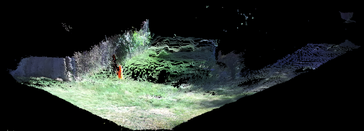
Because this sensor does not use structured light, it is not as affected by bright sunlight. There are still a few issues that need to be worked around, which will be discussed in the algorithm section below, but the sensor is very stable and consistent. In addition, it is able to leverage the GPU inside the TX2 to deliver point clouds in real-time (e.g. < 30ms) with minimal CPU Usage.

Algorithm

Once the sensors capture the environment, the data is forwarded to the perception algorithm. The perception algorithm works by dividing up the world into a 2-d grid, or “occupancy matrix.” Each grid square will be categorized into one of a few categories: TRAVERSABLE, UNTRAVERSABLE, UNKNOWN, or CONE. The latter is a special type of untraversable terrain which has been identified as the goal. The input to this algorithm is the point cloud generated by the ZED2, and the output is the 2-d occupancy matrix.

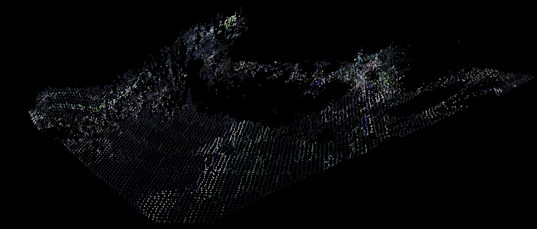
The algorithm operates in a few distinct steps. First, it starts by consuming the full input point cloud from the ZED2:

The point cloud is extremely dense, containing over 900,000 points! Although this gives a very detailed view of the surface, it can be difficult to process in real time. In addition, the point cloud can be noisy, especially when dealing with rough surfaces like gravel and grass. As a preprocessing step, the algorithm utilizes voxel grid downsampling. This step divides up the 3-d space into discrete “voxels”, or cubes. It then collects all of the points that fall into the cube, and replaces those points with a single point formed from the centroid. The output of this step is a much less dense point cloud that still maintains the original structure.

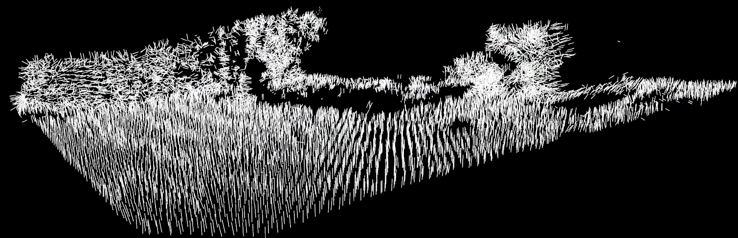
In order to distinguish traversable terrain from non-traversable terrain, a variety of strategies can be used. One popular technique is to attempt to fit a “ground plane” to the points. While this works well in indoor environments, this fails in outdoor environments because the ground is generally not perfectly flat. Instead, the algorithm considers the normals of each point. For points on a plane that is perfectly flat, the normals will point straight upwards. However, if the points represent a wall, then the normals will point sideways. By using this information, it becomes possible to segment the point cloud into “traversable” and “untraversable” regions. The normals can be computed using the GPU, so the computation is quite quick. In the picture below, the white lines represent the normals. Notice how for the traversable regions, they all point “pretty much upward”, and they sharply change direction at obstacles.

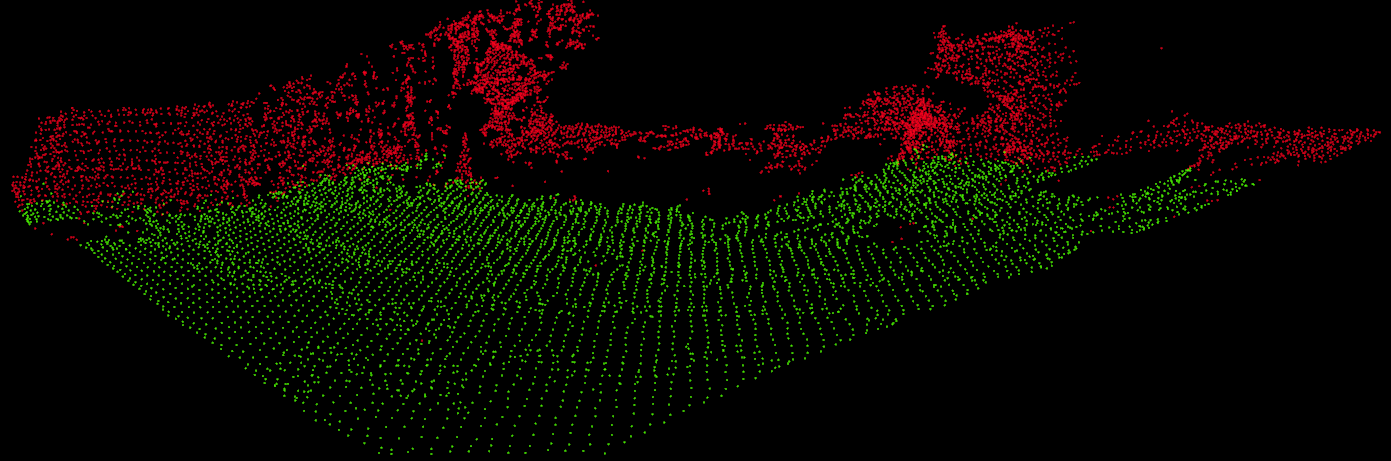
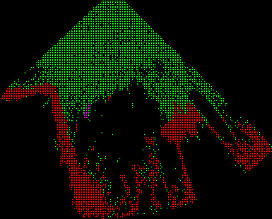
Once the normals are computed, the points can be classified as “traversable” or “untraversable”. The algorithm does this via a breadth-first search, starting with all points in a small neighborhood around the base of the robot. For each traversable points, the difference in normals between the point and its neighbors are checked. If the difference is small, and global thresholds are met, then the neighbor will be marked as traversable, and the process continues. Below is a visualization of the point cloud after segmenting. The red points are deemed untraversable, while the green points are traversable.

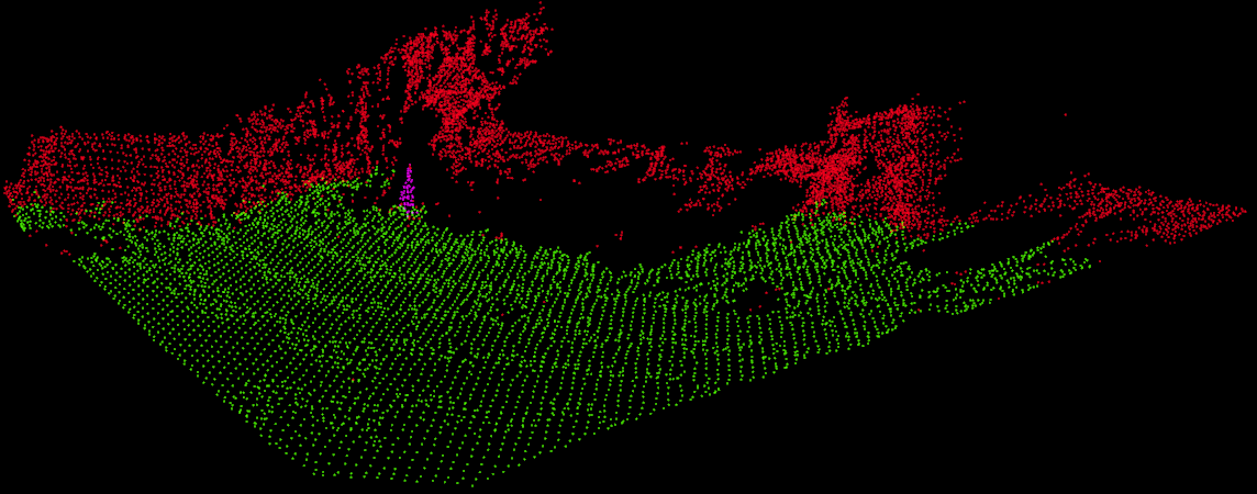
After identifying the untraversable regions, the untraversable regions are then examined for cones. Cones are primarily identified by their distinctive orange color. The RGB color is swapped to HSV space and thresholded. Neighboring points are then collected into clusters, and examined. If the clusters are large enough and of the proper shape, they are marked as a cone. The visualization below shows the algorithm after the cone detection portion runs. It is identical to the cloud above, but some of the untraversable points have been identified as a cone, and thus are marked in purple.

Finally, once the cloud has been fully processed, the occupancy matrix is generated. This is done by simply dividing up the space covered by the point cloud into discrete blocks, and having each block vote on its status. The block with the most votes determines the status. For example, if there are 10 points in a given region, 6 of which are untraversable, and 4 of which are traversable, the occupancy grid will mark the square as untraversable. In addition, if a square has too few votes, it will be marked as “unknown.” This can often happen if the point cloud has a region for which it fails to retrieve depth (e.g. from occlusions). The final output is shown below.

Miscellaneous Notes

There are a few interesting points to note about the algorithm

• On the TX2, the algorithm runs at approximately 5-10 frames per second for a 1280x720 input point cloud. The step that takes the longest is the initial voxelization of the point cloud, mainly because PCL does not have a GPU-ready implementation (n.b. there is a GPU implementation in the library, but it is unmaintained and probably broken. It currently doesn’t compile).
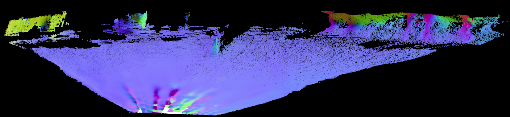
• The ZED2 does have an API to get surface normals. We cannot use it here for two reasons. First, after voxelization, the correspondance between normal and point is lost. Second, the ZED2 appears to return weird values for surface normals. Shown below is a colorized version of the output of this API - the points are shown in XYZ space, and the colors represent the normals. Notice how for the flat region near the base of the bot, there is a large variance in the computed normals. This appears to be an artifact of their algorithm, which is closed-source and cannot be investigated further :(.

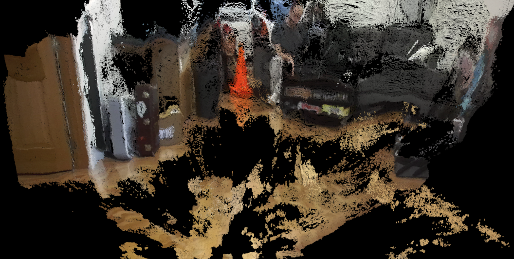
• The ZED2, like most stereo cameras, does not do well with reflective surfaces. One of the constant pain points of development were the hardwood floors in my apartment - the ceiling lights would cause glare which would translate into “holes” in the ground. This can be seen in the point cloud below. This is exacerbated when the camera is near the floor - hence the reason the camera is raised up.

Localization

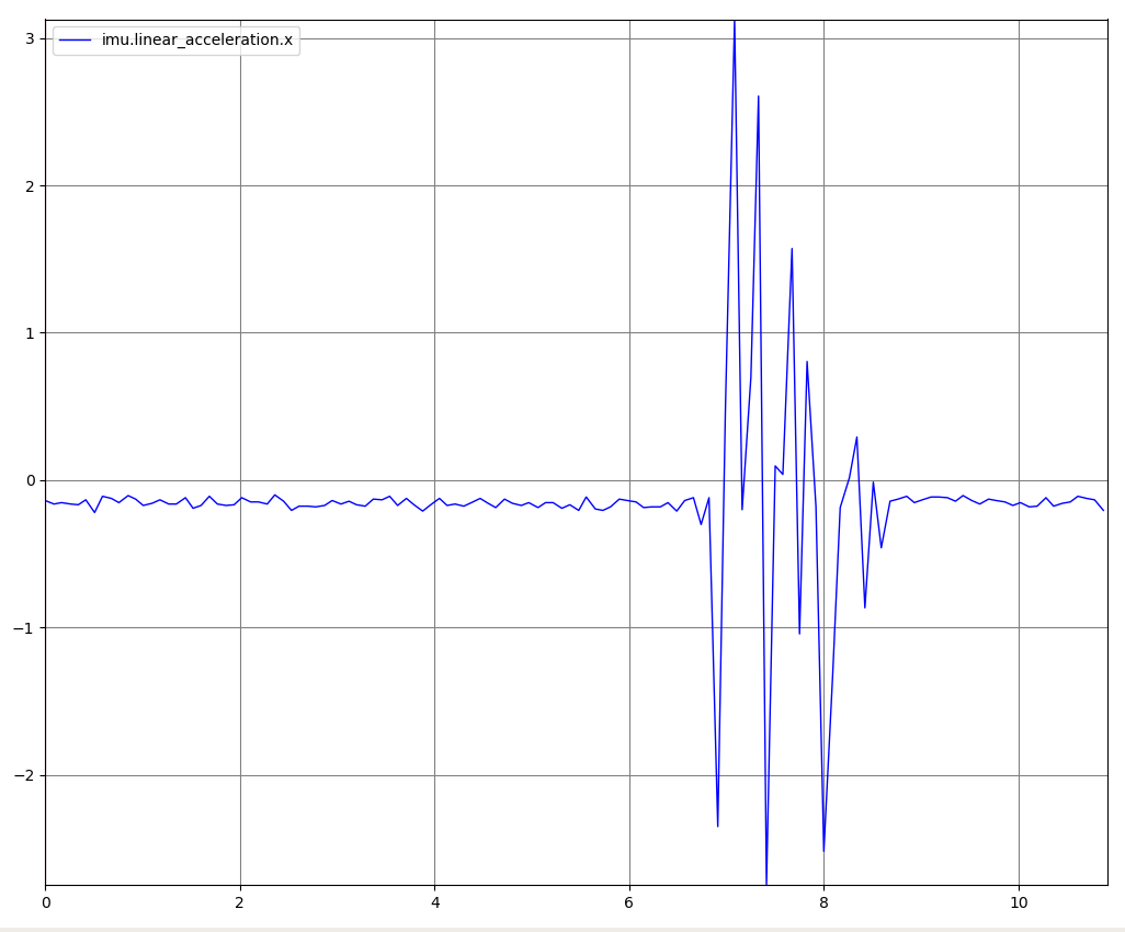
In addition to knowing the local obstacle field, the robot needs to know where it is located. Without this information, it will be unable to plan a path to its goal. The initial idea was to use the on-board IMU and GPS to form a kalman filter. However, this tended not to work too well for two reasons. First, the GPS unit did not have high enough resolution to reliably track the position of the bot. This is to be expected, as most hobby GPS sensors give accuracy down to a few hundred feet at best. The more suprising failure was the IMU - while the IMU appeared to yield reliable data when the bot was stationary, every time it began to move erratic spikes in the data were seen:

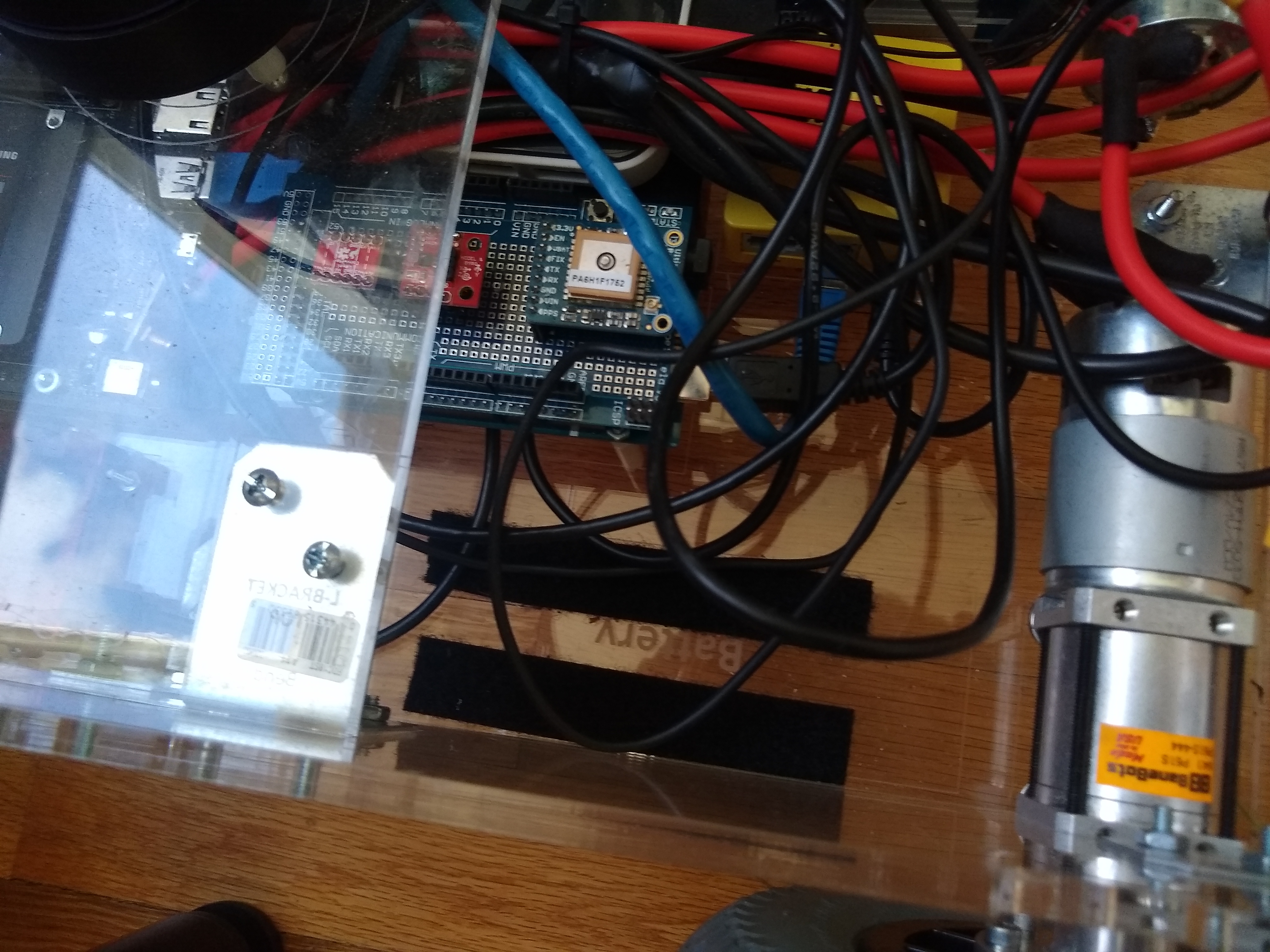
It turns out that the location of the IMU is problematic. The IMU selected is a piezoelectric device, meaning it works by amplifying small microelectric charges. Unfortunately, it is located directly next to one of the motors - the IMU is the red chip in the center of the blue PCB on the left in this photo:

The motor interference corrupted the data returned from the IMU, making it pretty much unusable. A few shielding methods were attempted without success.

In addition to the IMU, there was a downward-facing webcam mounted on the bottom of the robot. The initial idea was that the robot would be able to track its position via optical flow, similar to the method used by optical computer mice. Unfortunately, the images retrieved from this camera turned out to be too blurry to be of any use - it was impossible to get accurate trajectory vectors when the camera was mounted so close to the ground.

Luckily, the ZED2 provides Visual Inertial Odometry (VIO) pose tracking. By utilizing the video feed and the onboard IMU, the ZED2 is able to keep track of the position of the sensor. Initial tests showed that this worked quite well for short (i.e. < 5 minute) periods of time, so this method is used for localization.

Planner

Once the robot’s location is known and the local obstacle map is known, enough information is known to determine the action to take. The planner module is responsible for this step of the pipeline. It accepts the occupancy matrix from the perception stack and the pose from the localization stack, and outputs control signals to the robot. In order to determine the correct signals to output, it begins by updating a global occupancy grid from the local occupancy grid received from the perception stack. When conflicting information is received, the algorithm favors the fresh information over the cached information.

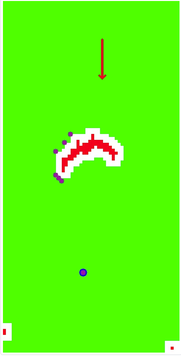
Once the global grid is updated, the planner uses the grid to plan a path. Because there are relatively few stationary obstacles in the environment, the planner can be quite simple. First, it treats the robot as a point object, and expands the bounds of each of the detected obstacles to create a “safety margin.” Then, the algorithm uses A* to plot a path from the robot’s current location to the goal using the L1 distance to the goal as the heuristic. After the path is plotted, a post-processing step is used to simplify the path, removing unnecessary points and reducing the path to the minimal set of straight lines needed. Shown below is a debug visualization of the path planned. The green squares are clear squares, the red are detected obstacles, the blue circle is the goal point, and the white squares are the expanded obstacles. The purple dots are the waypoints of the computed path, and the arrow represents the current location and orientation of the bot.

A* can be used beacuse the world of the bot is relatively small, and the obstacles are static. So the path does not change very often, and if it does, the world is small enough that recomputing it is quick. In addition, because the obstacales are static, the path can be cached after being computed the first time, and only updated if it is later found to be invalid. After the path is planned, it is a simple matter to compute the control signals necessary to drive the robot towards the desired waypoint. The heading of the bot is compared to the heading needed to get to the goal point, and this ratio is used to compute the amount of torque to apply to the left and right motors.

Robot Devops

The success of any algorithmic work depends on a base of solid engineering fundamentals, and this robot is no exception. From data collection to interface design, there were a wide variety of challenges that needed to be solved in order to get the robot to an operational state. There are a few points of interest worth discussing related to engineering and running the system, or “robot devops”:

Ensuring Safe Operation

Robots are expensive and contain lots of high-power, high-voltage components. It should be made as difficult as possible to run the robot in a configuration in which it can cause injury to itself or others. There are a few layers of safety baked into this robot. The first layer of protection involves the electrical system discussed in the previous post. With that system, it becomes impossible to overdraw the batteries, eliminating a major source of concern.

Another potential issue would be disconnection or misidentification of hardware devices. There could be major problems, for example, if the left motor controller was misidentified as the right motor controller. This is made more complicated by the fact that there are many USB devices plugged into the system, and they are assigned random identifiers at startup. That is, on one bootup, the left motor controller might have the device identifier /dev/ttyACM0, and on the next /dev/ttyACM1. The solution is a build-time python script that attempts to communicate with each device. If successful, it generates the launch files with the device identifier. This means that the robot cannot be run if the hardware is disconnected, solving this potential problem.

Data Collection

One of the initial reasons for choosing ros as a framework was that it allowed for easy data collection and replay via the rosbag tool. This tool attaches to incoming and outgoing topics, recording data to a “rosbag” file. These rosbags are convenient to work with in the ros ecosystem, allowing real-time replay of the data back onto topics. In addition, there are a variety of tools that can be used for examining the data contained within the rosbag, such as rviz or rqt_bag.

That’s the pitch. In reality, there are complications:

• Rosbags grow large really fast. They also don’t adapt to changing schemas well - if message types are changed, then the MD5 hash of the type changes, and the rosbag cannot be used. It quickly becomes a mess keeping track of which types are used as schemas evolve.
• Recording rosbags are inefficient and CPU intensive. This isn’t as big of a deal when the contained data types are small - things like floats or poses. But, the system starts to significantly slow down when recording images, and completely falls apart when attepting to store point clouds.
• The tooling isn’t very good. Rqt_bag is fine for quick examination, but doing custom plots or deep analysis is difficult. Plus, it can only visualize very simple types out-of-the-box, such as time distributed floats. There is a plugin system, but it is complicated to use. In addition, rviz has severe performance problems when attempting to display larger data such as point clouds. It turned out to be completely unusable for this application.

A lot of time was spent attempting to develop a robust data capture system using rosbags. Eventually, writing a series of custom data collection tools and debug visualizations turned out to be much more fruitful than attempting to use the open source tools. The lesson here is twofold. First, while it is a good idea to plan ahead for data collection needs, one should verify that the data is necessary before spending the engineering effort to design the collection system. The second lesson is that time spent developing custom debugging tools is usually worth it, as it is generally paid back tenfold when attempting to get the system to work. The debug UI generated for the planner and the point clouds were essential in debugging the operation of the system, and took a few days of development. In contrast, the rviz visualizers took weeks of boilerplate piping code to use the “free, out-of-the-box” visualizers, and turned out to be entirely useless.

Future work

There are plenty of areas for future improvement in the robot:

• Perception: While the method for determining traversability appears to be quite solid, the cone-detection capability is a bit more flakey. Currently, it uses shape and color heuristics, which are not always reliable in all environmnets. Ideally there should be some sort of machine learning model that will process the point cloud and detect cones; however, that would require collecting a large amount of data.
• Localization: The localization from the ZED2 appears to be stable over short distances, but it does not fare well during long drives. The values tend to drift, becoming noticably inaccurate at around 5 minutes into the run. This is problematic because it is the robot’s only form of localization. A future extension would be to use additional cameras or better LIDAR sensors to provide additional points of reference.
• Path Planning Improvements: The current algorithm uses A*, which works and is provably optimal. However, if the robot is to travel for longer distances, then it will consume too much compute to be used in real time. There are more advanced path planning algorithms such as D* which could be explored. In addition, the path planning algorithm assumes the robot is a point obstacle, and expands the obstacles to provide a safety buffer. This works for this problem because there are few obstacles. However, with more obstacles, it could become possible that the robot would be unable to find a valid path because it is being too conservative in its planning. To fix this issue the dimensions of the robot will need to be taken into account, potentially by using a higher-dimensional path planning space.
• Simulation integration: Initial work was done with integrating the platform with UrdfSim. While the infrastructure has been laid, there will need to be more work done in order to use the simulator with the current setup, as the ZED2 sensor is not currently supported by UrdfSim. In general, the value of simulation for this particular problem is low, as most of the problems found during development were ones with the physical hardware or capabilities of the sensor - they would not have been able to be found via simulation.
• Devops: While there are hooks for making the entire system configurable, there isn’t a nice UI developed. In addition, the robot currently only supports traversing to a single destination. To solve the robo-magellan competition, the process would need to be repeated for multiple waypoints.

Summary

In this experiment, the teleoperated robotic platform was extended for autonomous operation in outdoor environments. A robust perception and localization stack was developed based on the ZED2 stereo camera, which is capable of detecting obstacles in real time using the TX2’s onboard GPU. Care has gone into the development of the deployment system to ensure that the robot can only operate when it is healthy, decreasing the liklihood of a catestrophic failure. This control system can serve as the baseline for more complex algorithms and experiments, which may allow the robot to operate in a wider variety of environments. The robot design files have been open-sourced, and can be found on github here. Here’s a short video of the robot in action!

Download Links

• Robot Development Repo. This contains the source code for the control system, build system, the bill of materials, and the design files for the chassis.