Introduction

Reinforcement learning is one of the popular methods of training an AI system. Rather than attempting to fit some sort of model to a dataset, a system trained via reinforcement learning (called an “agent”) will learn the optimal method of making decisions by performing interactions with its environment and receiving feedback. One of the first algorithms introduced in this area was the Q-Learning algorithm. First introduced in 1989, the algorithm involves the agent experimenting with the environment, and receiving a reward for each action. Over time, the agent will learn the optimal actions to take in order to obtain the largest amount of award. The beauty of this algorithm is that is is completely domain agnostic - the “actions” and “rewards” could be anything, allowing the algorithm to be easily ported across domains

In this blog post, we’ll dissect the classic Q-Learning algorithm, and use it to solve a simple problem. Along the way, we’ll discuss the strengths and weaknesses of this algorithm, and how it can be modified for more complex scenarios.

The Q Learning Algorithm

In most reinforcement learning algorithms, the agent is modeled as a finite state machine. That is, there are a finite number of possible states, s, in which the agent can reside. At each iteration, the agent must take an action A(s, s’), which transitions the agent from the current state s to a new state s’. Depending on the problem, the agent may be able to move between any two states s and s’, or there may be restrictions making some choices of s and s’ invalid.

When moving between any two states, the agent receives feedback from the environment in the form of a reward R(A(s, s’)) (this should be read as “the reward of taking the action of moving from state s to state s’”). The objective of any reinforcement learning algorithm is to maximize the value of this reward function over time.

In Q Learning, this task is accomplished by utilizing the learning matrix, Q(A(s, s’)) (hence the name ‘Q-Learning’). Q represents the agent’s long-term expectation of taking action A(s, s’). Once trained, the agent can use this Q(A(s, s’)) matrix to determine which action to take by selecting the state s’ which maximizes Q(A(s, s’))|_s (read that as “maximizing the expected long-term reward from taking the action A(s,s’) moving the agent from state s to state s’ given that the agent is currently in state s”). This means that once the learning matrix is trained, the agent will be able to determine the optimal action from any state.

Ok great, so how do we train this Q(A(s, s’)) matrix? The simplest method is through iterated applications of the Bellman Equation. In plain English, the idea is that we begin by initializing the matrix to zeros, so that all actions have equal weight. Next, we place the agent in a random state, and allow it to wander around throughout the environment randomly. After each decision, we then update the Q matrix using the Bellman Equation:

Q(A(s,s’)) = R(A(s,s’)) + (gamma * Max_s’’|s’(Q(A(s’, s’’))))

There are a few new symbols to discuss in this equation. The first is this s’’ character. Similarly to how s’ represents the “next state” given the current state s, s’’ represents the state after the next state s’. Another way of wording it is that s’’ is a move that is two actions away from the current state s. It is used in the last term in the expression, Max_s’’|s’(Q(A(s’, s’’))). While this expression looks intimidating, what it is saying is “find all of the expected rewards for the actions transitioning the agent from state s’ to state s’‘, and take the maximum”. This term is a way of allowing the agent to consider rewards from future moves rather than just optimizing for the decision at hand. For example, consider teaching an agent to play chess. If this term were absent, then the agent would always make the move that would capture the highest ranking piece. This would be a very poor agent - it would fall for any trap or gambit, because it would be unable to look two or three moves ahead into the future to see a trap!

Having discussed the importance of the final term, the importance of gamma, or the “discount factor” becomes clear. It represents the amount of weight the algorithm should put on future rewards over immediate rewards. Notice that if gamma == 0, then the learning algorithm reduces to simply Q(A(s, s’)) = R(A(s,s’)). While this may work for simple problems, usually gamma takes the value 0 <= gamma <= 1 to allow the model to consider future actions at each decision juncture.

If the agent happens to reach a terminal state (solves the puzzle, crashes the car it’s learning to drive, etc.), we then reset the agent to a random state and continue the process. We continue to update the Q(A(s,s’)) matrix until further updates do not cause the existing values to change much. At that point, we’ve said that the matrix converges, and that the agent is trained. For the mathematically inclined, it can be proven that this algorithm will eventually converge.

Now that we have a solid understanding of the basic Q Learning algorithm, let’s take a look at how we can use it to solve a simple problem - a maze.

Application to Maze Solving

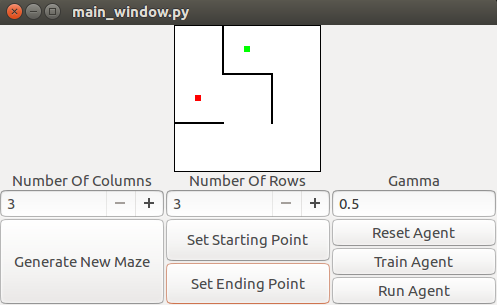
In our problem, we have a maze of constant, fixed size with r rows and c columns. The maze is composed of blocks, which may or may not have walls between them. Blocks are connected to each other on the top, bottom, left, and right edges, except when either the block is on the outer edge of the maze, or there is a wall between the two blocks. The walls are randomly generated at maze generation time, and are static throughout the learning and testing processes. The maze also contains a goal point. The agent we are training will be given a starting point, and must determine the shortest path from that starting point to reach the goal point. It is guaranteed that such a path exists. Below is a visualization of the maze. In the below maze, there are 9 blocks arranged in a 3x3 square (that is, r==3 and c==3). The goal point below is shown in green. A potential starting point is shown in red.

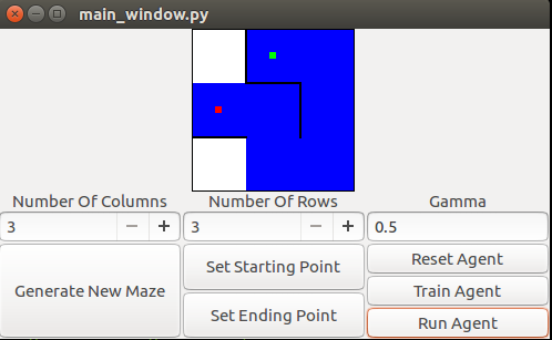
The agent would be expected to produce the path shown in blue

While maze generation is an interesting topic in and of itself (and if you check out the included code, you’ll see that it’s not a trivial task =P), let’s assume that we have a representation of the maze M. We first need to decide how to represent the states. In this case, a reasonable representation is to give each block a number. We’ll arbitrarily choose to number the states starting at the top left, in row-column format. That is, the top-left block is state 0, the block to the right is state 1, etc. For a maze with r rows and c columns, there are then r*c states. Then, we can represent both the reward R(A(s,s’)) and expected reward Q(A(s,s’)) as rxc by rxc matrices.

The next step is to decide how we want to reward the agent. The desired behavior is that the agent reaches the goal, and stops. Also, we need to identify the restrictions on A(s,s’). There are two restrictions to be cognizant of. First, unless the agent is at the goal, it may not remain in the same state between to iterations. Thus, we may not allow A(s,s) to be chosen ever. The next restriction is that if there is a wall between two blocks, or if the move would cause the agent to move outside the edges of the maze, then the move is invalid. Given this, we can initialize our R matrix:

  def reward():
    if (action_moves_agent_to_goal_state):
      reward = 1
    elif (action_is_valid):
      reward = 0
    else:
      reward = -1

For the maze in the image above, the R(A(s,s’)) matrix looks like this:

[-1., -1., -1.,  0., -1., -1., -1., -1., -1.]
[-1.,  1.,  0., -1., -1., -1., -1., -1., -1.]
[-1.,  1., -1., -1., -1.,  0., -1., -1., -1.]
[ 0., -1., -1., -1.,  0., -1., -1., -1., -1.]
[-1., -1., -1.,  0., -1., -1., -1.,  0., -1.]
[-1., -1.,  0., -1., -1., -1., -1., -1.,  0.]
[-1., -1., -1., -1., -1., -1., -1.,  0., -1.]
[-1., -1., -1., -1.,  0., -1.,  0., -1.,  0.]
[-1., -1., -1., -1., -1.,  0., -1.,  0., -1.]

The Q(A(s,s’)) matrix starts out as zeros, as we don’t know anything about the maze initially.

To train the matrix, we will begin by placing the agent in a random state s. We’ll then get a list of the next possible states by looking at the R matrix - if the value for R(A(s,s’)) is < 0, then the movement is invalid and may not be chosen. Of the valid moves, we randomly pick a next state s’. Given that next state s’, we look at all values of Q(A(s’,s’’)) for all valid A(s’,s’’), and take the maximum. We then combine that with the reward function R(A(s,s’)) as determined by the Bellman Equation, and update the value of Q(A(s,s’)). In pseudocode, the algorithm looks like this:

  def train():
    while(not_converged()):

      # Start in random state
      state = get_random_state()

      # Keep going until the goal state is reached
      while(state != goal_state):

        # Pick a random next state
        possible_next_states = get_valid_next_states(state)
        next_state = random.choice(possible_next_states)

        # Get the best Q Value over all valid actions from the next state
        next_next_states = get_valid_next_states(next_state)
        max_q_next_states = max([Q[next_state][s] for s in next_next_states])

        # Update the Q matrix
        Q[state][next_state] = R[state][next_state] + (gamma*max_q_next_states)

        #Move to the new state
        state = next_state

Here’s what the trained Q matrix looks like for the maze above (n.b. the entries have been rounded to 2 decimal places for readability):

[ 0.00, 0.00,  0.00, 0.26, 0.00, 0.00, 0.00, 0.00, 0.00]
[ 0.00, 0.00,  0.00, 0.00, 0.00, 0.00, 0.00, 0.00, 0.00]
[ 0.00, 1.00,  0.00, 0.00, 0.00, 0.64, 0.00, 0.00, 0.00]
[ 0.21, 0.00,  0.00, 0.00, 0.33, 0.00, 0.00, 0.00, 0.00]
[ 0.00, 0.00,  0.00, 0.26, 0.00, 0.00, 0.00, 0.41, 0.00]
[ 0.00, 0.00,  0.80, 0.00, 0.00, 0.00, 0.00, 0.00, 0.51]
[ 0.00, 0.00,  0.00, 0.00, 0.00, 0.00, 0.00, 0.41, 0.00]
[ 0.00, 0.00,  0.00, 0.00, 0.33, 0.00, 0.33, 0.00, 0.51]
[ 0.00, 0.00,  0.00, 0.00, 0.00, 0.64, 0.00, 0.41, 0.00]

Once trained, we can solve the maze from any starting point easily by taking the maximal value of Q(A(s,s’)) for any given state until we reach the goal. In pseudocode, the algorithm looks like this:

  def solve(state):

    # Initialize path
    path = []
    add_state_to_path(state)

    # Keep going until goal state is reached
    while(state != goal_state):

      #Get all possible next states
      possible_next_states = get_valid_next_states(state)

      #Pick the state that maximizes Q[state][next_state]
      best_next_state = argmax(possible_next_states, lambda ns : Q[state][ns])

      #Move to that state and add it to the path
      state = best_next_state
      add_state_to_path(state)
    return path

For example, in the maze above, the agent is initially in state 3. The agent can go to either state 0 or state 4. We compare the Q(A(s,s’)) values for both of those moves by looking at the Q matrix: Q[3][0] == 0.21, and Q[3][4] == 0.33. Because Q[3][4] > Q[3][0], the agent selects A(3,4), and moves to state 4. From state 4, we can move to either state 3 or state 7. Q[4][3] = 0.26, and Q[4][7] = 0.41, so the agent chooses A(4,7), and moves to state 7. The process is repeated until we reach teh terminal state, state 1, giving the final path [3,4,7,8,5,2,1].

The Application

The algorithm describe above has been implemented in python. The code can be found on github here. The GUI was developed using the glade GTK editor, and the application uses PyGTK to display it. The meat of the Q Learning algorithm described above is implemented in the qlearn_agent.py file. Some minor implementation details:

• Because the list of valid moves from each state to each new state do not change over time, they are cached once in a hash table. This is merely a performance optimization, and does not change anything about the core algorithm.
• In order to prevent the values in the matrix from becoming to large, the matrix values are periodically normalized. That is, each entry is divided by the largest value in the matrix, so that Max(Q(A(s,s’))) == 1.0
• The app has been tested to work on Ubuntu Linux 14.04 and 16.04 with python 3.4. It depends on PyGTK and numpy. It should work on other platforms, but hasn’t been tested. If you do find bugs, let me know in the comments and I can try to fix them :P
• During testing, the situation was occasionally observed in which the same point was chosen twice as a starting point. This sometime caused premature convergence, as taking the same path twice through the maze wouldn’t change Q. To fix this, we only consider stopping after reaching the goal 10 times from 10 random starting points.

The logic for generating and drawing the maze is contained within maze.py. It’s a general-purpose maze generator that can be re-used for other purposes (e.g. you may see a pathfinding blog post soon :P). All of the wiring is contained inside main_window.py. It’s a great example of how to use glade to generate simple GUIs to use with python programs. To run the program, type from the command line

python3 main_window.py

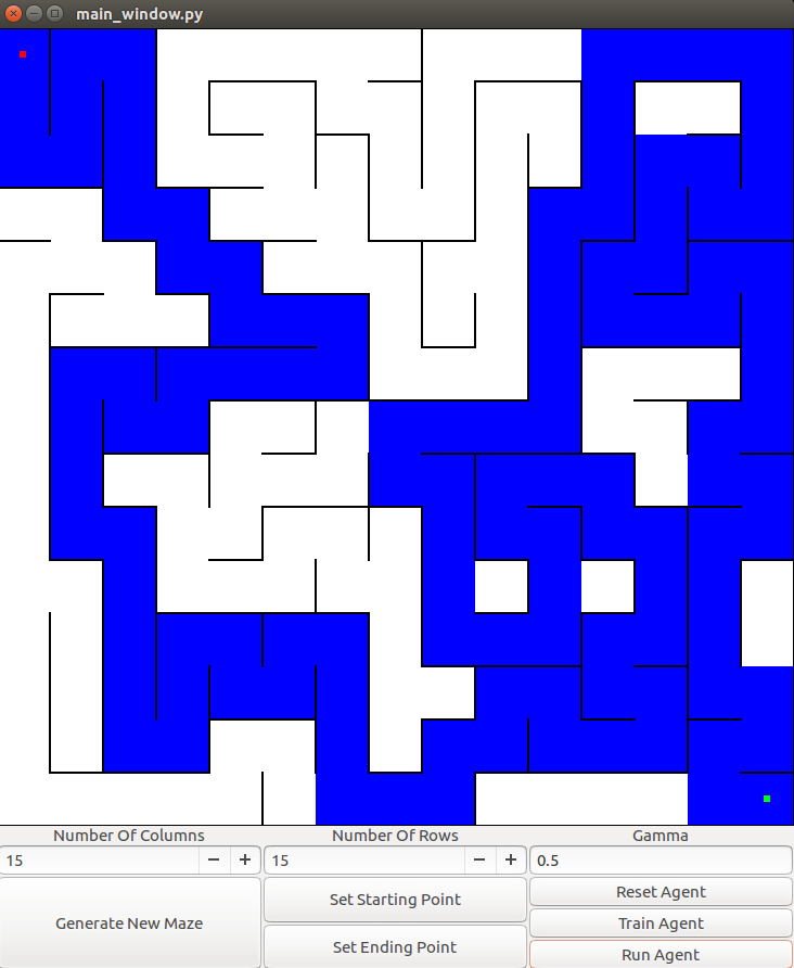
Although we used a 3x3 maze in the example above, the algorithm scales to larger mazes. Here’s an example of it solving a 15x15 maze:

Benefits and Drawbacks of Q Learning

Q Learning has many benefits over other traditional machine learning algorithms:

• The algorithm is completely generic. There is nothing that is really tying it to mazes specifically, it can be re-used in other applications easily.
• No previous knowledge is assumed about the environment (maze)
• No training data is needed - the algorithm learns organically
• After training, the optimal action for each state is known
• The algorithm is mathematically guaranteed to converge

There are a few drawbacks to this approach:

• The algorithm can spend a lot of time running through random states searching for the terminal state.
• The amount of memory required to store the Q matrix grows as (number_of_states^2). For mazes, the number of states is relatively small (e.g. hundreds). But consider trying to train a Q learning algorithm to operate a bulldozer. There are tons of state variables to keep track of, and each has many values. Thus, the number of states explodes exponentially, requiring lots of training time and memory.
• The reward matrix is assumed to be static. If the maze changes, or the goal changes, the agent needs to be retrained from scratch.
• The agent will always take the optimal path. This doesn’t allow it to adapt or learn new strategies. In this example, the ability to adapt is unnecessary, as the maze is static. But if the maze were not static, the agent would always attempt to take the same path between two points. A variant of the algorithm, called epsilon-greedy has the user choose an action A(s,s’) at random epison percent of the time, and the optimal action 1-epsilon percent of the time. Typically, epsilon is small (e.g. <0.05), but this allows the algorithm to occasionally explore and find new, more optimal solutions to the problem at hand.
• Sometimes, the Q(A(s,s’)) value can oscillate between different values. To combat this, sometimes algorithms introduce a learning rate parameter alpha which takes a value on the range [0, 1]. Instead of directly assigning the value of Q(A(s,s’)), the new value will be computed as Q(A(s,s’)) = Q(A(s,s’))|_old + (alpha * Q(A(s,s’))|_new). This causes the algorithm to converge more slowly, but can be more stable.

There is a variant of Q Learning that is becoming popular in which the values of Q(A(s,s’)) are predicted via a deep convolutional neural network. This approach, called “Deep Q learning,” has shown great promise, combining the best of deep learning and reinforcement learning algorithms. For more information, a good overview can be found here.

Summary

In this post, we used the classical Q Learning algorithm to solve a simple task - finding the optimal path thorugh a 2 dimensional maze. While implementing the algotirhm, we discovered some of the benefits and drawbacks to using Q Learning to solve AI problems. This simple algorithm is suprisingly versitile, and is one of the hottest topics in the AI community today.