Introduction

Matrix factorization is the act of decomposing a matrix into the product of two or more matrices. Matrices appear all over the place in data science applications. For example, the input to many classical models such as random forest is generally a structured two-dimensional dataset, with the columns representing the different features and the rows representing the samples. This dataset can be thought of as a two-dimensional matrix. Many popular algorithms leverage matrix factorization in an attempt to solve tasks ranging from data cleaning to label prediction. In this post, three use cases for matrix factorization will be examined. First, the Singular Value Decomposition (SVD) will be explored. This algorithm leverages matrix factorization to find a low-rank representation of a dataset. This can potentially allow for the elimination of features, decreasing the chance of model overfitting and the required amount of training data. Next, this post will explore two matrix-based approaches to building a recommendation system - Alternating Least Squares (ALS) and Gradient Descent (GD). The code for all of these examples are available in executable python notebooks available on github.

Singular Value Decomposition

When collecting a dataset, it is often represented in terms of human-recognizable features. For example, a dataset that describes computer hardware might have columns for the number of cores, the amount of ram, and the CPU clock speed. However, usually the features are not all totally independent. For example, a CPU with more cores generally has more RAM as well. This means that rather than describing the dataset with N features, it may be possible to describe it with K features, where K < N. If this transformation exists, it would be desirable to find it because it will reduce the amount of input features to the model, which would in turn decrease the model’s tendency to overfit and decrease both the training time and amount of samples needed.

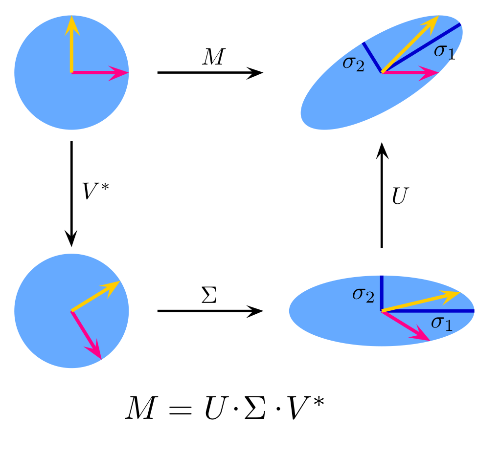
The Singular Value Decomposition works by taking a matrix M and decomposing it into three special matrices, U, S, and V such that M = U * S * V. In addition to this constraint, U, S, and V have special properties:

• U and V are both unitary. In the general sense, this means that U^†U = V^†V = I. For the real-valued matrices that are generally encountered in data science, this reduces to U^TU = V^TV = I.
• S is diagonal matrix, where the diagonal elements are strictly decreasing. That is, s₁₁ ≥ s₂₂ ≥ … ≥ s_nn

In more intuitive terms, U and V represent rotation matrices that do not “stretch” the space, while S represents a matrix that “stretches” the space without rotating it. The Singular Value Decomposition is trying to transform an arbitrary linear transform into a rotation, stretch, and another rotation. The image below from Wikipedia does a great job of visualizing the purpose of these three matrices:

The question may arise as to how this process is useful in data science. The answer likes in the S matrix. The elements in the S matrix show the relative stretching of the space in each of the directions pointed to by the V matrix. If a direction has very little stretching, then that means that that dimension has little discriminative power, and can be safely ignored. When performing the SVD on a dataset, it is not uncommon to find that greater than 95% of the variance is explained in the first few dimensions! This gives a straightforward algorithm for extracting a low-dimensional representation of a dataset: perform a SVD and take a look at the values in S (often called the ‘singular values’). Remove the dimensions that have small singular values. The remaining dimensions expose the low-rank representation of the dataset.

It is helpful to illustrate the power of the SVD with two examples. First, consider a toy dataset with low rank structure:

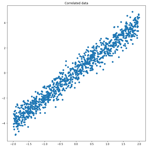
Here, the dataset is strongly correlated around the line y = 2x. When we perform the SVD, we see that the two singular values are 83 and 7. This means that the first dimension contains nearly 12 times the variance of the second dimension! The dimensions corresponding to the singular values appear in the columns of V, and are plotted below on the chart:

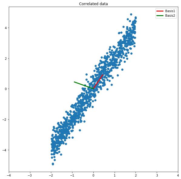
There are two important things to notice about the basis vectors:

• The basis vectors are perpendicular.
• The basis vector corresponding to the larger singular value points along the line y = 2x, as expected.

Using the SVD, we would be able to transform this dataset from a two-dimensional to a one-dimensional representation while still retaining much of the underlying structure.

As a more interesting application, consider an image compression task. A grayscale image is nothing more than a 2-d array of integers, so it’s possible to compute its SVD. After computing the images, we can then take a look at the singular values. Surprisingly, the bulk of the variance is contained in the first few singular values:

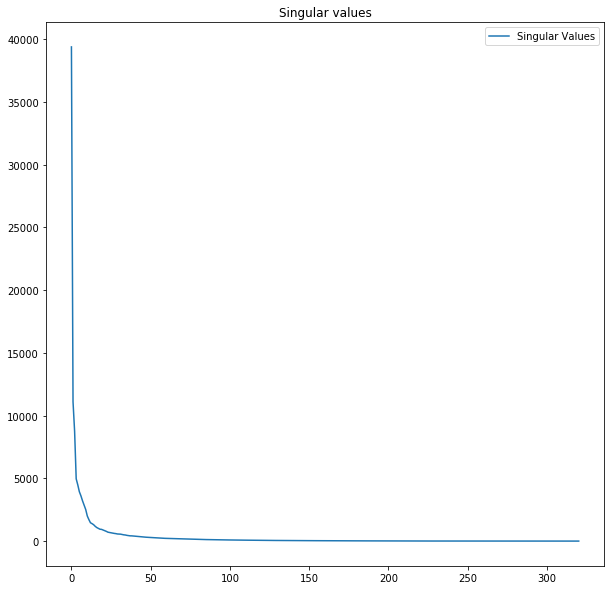
The implication of this is that by using relatively few basis vectors, it is possible to get an accurate reconstruction of the image. For example, here is an image reconstructed by the first N basis vectors:

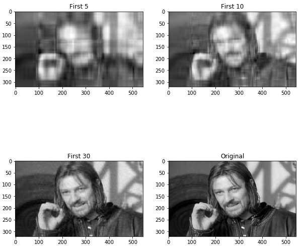
This fact is exploited by many popular image compression algorithms in use today, such as JPEG.

Recommendation Systems

One of the common applications of machine learning is recommender systems. Unlike classification or regression models, recommender systems are designed to use ratings or reviews provided by users to identify items that the users may be interested in. For example, a recommender system could be used to recommend movies that the user may like based off of their previous reviews. Recommender systems are a bit different from other modeling tasks because the structure of the input data is different. For many other tasks, such as classification, the dataset consists of a series of feature-label pairs. In a recommender system, the dataset consists of a user-item-rating tuple. The ratings are provided for only a small subset of the possible user-item combinations, and the purpose of the model is to infer the ratings for the user-item combinations that are not provided.

The examples below train a recommender system for the jester dataset, which consists of a series of 150 jokes that are rated by over 50,000 participants. One unusual aspect of this dataset is the fact that the density, or percentage of user-item combinations that have ratings is >22%, which is extremely high. Most datasets for recommendation systems have densities of less than 10%, while some have densities less than 1%. The high density makes it likely that our algorithms will be able to train with reasonable performance.

When thinking about recommender systems, the dataset is oftentimes described in terms of a ratings matrix, R. The ratings matrix is a matrix where the (u,i)-th element corresponds to the rating that user u gave to the i-th item. This means that the matrix has dimensions of U X I, where U is the total number of users, and I is the total number of items. The unrated elements are filled with a dummy value, which is generally 0. In both of the matrix factorization approaches below, this matrix is factorized into multiple sub matrices, which can then be used to generate predictions for the unlabeled spaces.

Alternating Least Squares

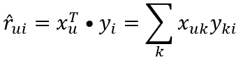
Alternating Least Squares takes the approach of factorizing the matrix into two sub-matrices, X and Y. X is of dimension U X K, and Y is of dimension K X I. Here, K is called the “latent dimension,” and represents the number of “latent features” that represent the user or item. Intuitively, this model says that each user can be represented by K attributes, and each item can be represented by K attributes. Further, it says that the user’s rating for an item can be approximated by the dot product between these two vectors:

Rather than attempt to guess what the attributes are, it is more practical to attempt to let the model figure them out by minimizing a loss function. Implied by the “least squares” part of the name, the primary driver of the loss function is the squared difference between the given and actual prediction (along with a few regularization terms):

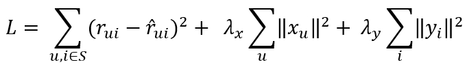
This is a function of multiple variables, but can be solved in an iterative manner - first by minimizing with respect to the user latent features, then by minimizing with respect to the item latent features. By alternating between these two optimization objectives, the algorithm will eventually converge on a solution that minimizes the squared error loss with respect to the training set.

This algorithm has a few nice properties:

• It is embarrassingly parallel. It turns out that the computation of the partial derivatives for each user is independent of the other users, and the computation of the partial derivative for each item is independent of the other items. This means that it would be possible to distribute the computation across multiple machines, making it possible to efficiently compute on large datasets.
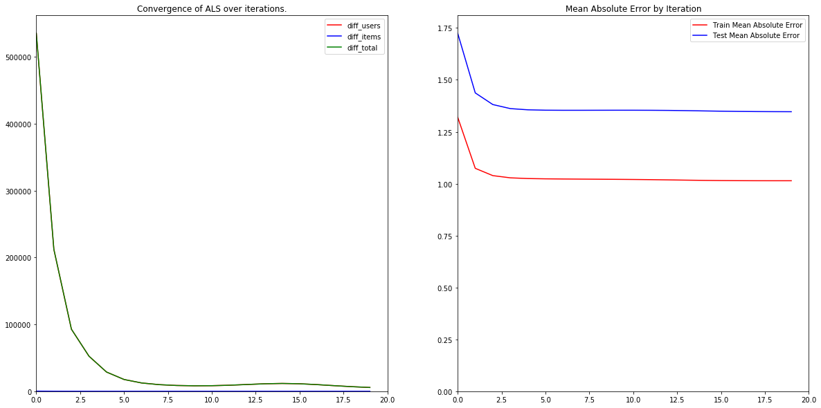
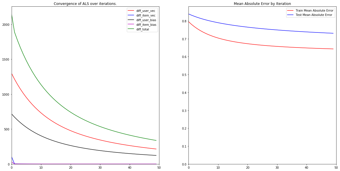
• It is robust to overfitting. Training for more iterations does not seem to increase the gap between training and testing accuracy.
• The algorithm converges relatively quickly. In our example, the loss was pretty much static (to within 1%) after 5 iterations.

Gradient Descent

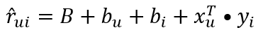
Although ALS is popular, there are other approaches to computing the user and item latent features. Another popular method is by using gradient descent. When using gradient descent, it is often a good idea to attempt to model the biases of the users and the items in addition to the specific user-item interactions. The user bias represents the likelihood that a user will give a high rating independent of the product that is being reviewed. The intuition is that some users are easy to impress, and will give high ratings for every item. Other users are hard to impress, and will give a low rating for every item. This term attempts to normalize the different rating scales. Likewise, the item bias represents the likelihood that a particular item will be highly rated regardless of the user that will be rating it. The intuition is that some items are objectively better than other items. Finally, there is an additional term for the global bias, which is simply the average rating across all items. When put together the new prediction function looks like this:

The loss function remains the same, with a few additional regularization terms added for the bias terms. Notice that the global bias is not part of the loss function - it is a constant.

To train this model using gradient descent, we use the standard backpropagation rule. Using this rule, we compute the gradient of the loss with respect to each variable being tuned (here denoted as V), and take a small step in the direction of the gradient. After taking many steps, the algorithm will converge on values for the user and item matrices that will minimize the loss:

This algorithm has a few benefits over ALS, as well as a few drawbacks

• The algorithm performed better. This is likely due to the addition of the bias terms.
• The algorithm took longer to train. In addition, it is not trivially parallelizable, as the global error is necessary to compute the backpropagation terms. This term depends on the predictions for all users and items, so it cannot be easily parallelized to many machines.
• The algorithm is prone to overfitting. Notice how towards the end, the training error continued to decrease, while the testing error remained constant. This is typical of gradient descent algorithms, and care must be taken to stop training once the testing loss has stopped decreasing.

In practice most recommender systems are composed of an ensemble of ALS, GD, and other models. This allows the overall model to benefit from the strengths of each model, while mitigating the errors caused by each individual model’s weaknesses.

Summary

This post introduced the concept of the Singular Value Decomposition, and showed how it could be used for dimensionality reduction and image compression. In addition, this post introduced the concept of a recommender system, and detailed two algorithms that can be used to build them - the Alternating Least Squares and Gradient Descent algorithms. All three of the techniques introduced in this post are forms of matrix factorization, in which a target matrix is decomposed into the product of two or more matrices. The code for all of the examples shown in this post is available on github.