Introduction

In the previous blog post on Q learning, we discussed the Q learning algorithm and applied it to a simple scenario. Recall that the Q learning algorithm operates in the context of an autonomous “agent” which is able to interact with its environment and receive rewards based upon its actions. Based on the rewards, the agent attempts to compute “Q” values for each of the possible actions at each state. Once it has computed the Q values, then the agent will take the action that has received the highest Q value overall. Recall that the Q values are defined by the Bellman Equation:

Q(A(s,s’)) = R(A(s,s’)) + (gamma * Max_s’’|s’(Q(A(s’, s’’))))

In the last post, we were able to compute the Q values exactly, which allows our agent to learn a provably optimal strategy for action selection. In this post, we will utilize Q learning to tackle a much more complex problem: Autonomous Driving. This task is much more complex than solving a maze; heavy modifications to the basic Q learning algorithm must be made. In particular, we will see that it is impossible for the algorithm to directly compute the Q-values for every state, so we must come up with a method of estimating them from state data. This gives rise to the deep Q network, the algorithm which we will explore in this blog post.

Problem Setup

One of the fundamental tasks that is required of an autonomous vehicle is road following. When a vehicle is on the road, it should be able to follow the turns of the road without running off the side. To isolate learning this behavior, we will make a few simplifying assumptions:

The car moves at a constant speed that will allow it to comfortably navigate all turns
The car is not traveling to a particular destination - that is, if it encounters a fork in the road, both paths are equally valid options
There are no moving obstacles in the road. That is, the environment is static.

Given these constraints, we can quickly define the different elements of our RL problem:

Agent: The agent will be the vehicle itself. For this example, we will be using an exeuctable built on Microsoft AirSim for our simulations, so the car that we pilot will be our agent. The executable can be downloaded from here (warning: large file!)
Environment: The environment will be all of the surroundings that the car will encounter while driving - the road, the walls, and the other present obstacles. We will use the “neighborhood” map of the AirSim executable, as it has a variety of static obstacles for our car to learn to avoid.
State: The state will be the sensor readings of the vehicle. For this task, we will start with the bottom-half of the image from the front-facing webcam. This can be viewed as a 59x256x3 dense tensor.
Action: For this problem, we will only be controlling the steering signal. While the steering angle is a continuous number between -1.0 (full left) and 1.0 (full right), we can simplify the problem drastically by only allowing the agent to select a few angles on that range. For this problem, we will allow the agent to choose between five steering angles: -1.0, -0.5, 0.0, 0.5, 1.0.
Reward: We want to reward the car for remaining on the center of the road. Thus, our reward function should give a high reward when the car is centered on the road, and a low reward when it’s driving on the sidewalk. Also, the reward function should be bounded on the range [0,1], as it will be easier for the network to learn a function on that range. Finally, the function should be continuous, as it is difficult to learn a function with discontinuities. A simple function that fits this criteria is a decaying exponential: R(s) = exp(-b * distance) where b is an arbitrary constant that controls how sharply the reward falls off (in the sample code, b = 3.5).

The Failure of the Classical Q Learning Approach and the Rise of the Deep Q Network

Now that we’ve defined the problem statement, we may be tempted to take the same approach to this problem as to our previous Q Learning experiment - building a lookup table for the possible actions that the agent can take and letting the agent roam freely until the values in the table stabilize. If we try that approach, we quickly run into a big problem: the number of states is massive! There are 59 * 256 * 3 = 45,312 possible states for the vehicle to be in. We’d need a 45kx45k matrix just to hold the Q values! Also, it is impossible for us to model the proper “next state” for each action - we don’t know a priori what the next state will be for any given action that we take until after we take it. Thus, we cannot guarantee that the agent is making valid moves whenever it is exploring the space. Unfortunately, this is not an issue that is unique to this setup - this problem makes it impossible directly computes the Q values for most real-world problems.

If we cannot compute the Q values exactly, another option is to attempt to estimate them. That is, we can train a model to predict the Q values for each action. Then, we can use the model output to determine which action to take at each state. Initially, the model will perform poorly, but over time, the predicted Q values will become closer to the actual Q values. Initial success was found using linear models for Q value prediction, but non-linear models generally had issues converging on an optimal solution. This limited the power of Q learning to simple problems that could be solved with linear models.

However, all of this changed with the introduction of the Deep Q Network (DQN) from Google DeepMind. In this paper, they showed that it was possible to train a deep neural network to predict the Q values. Their agent was tasked with playing classic Atari games, in which the inputs were frames from the game, and the actions corresponded to button presses. After exploring a few hacks, the agents were able to outperform humans on >80% of the classic Atari games! The network itself was nothing groundbreaking - it was just a few convolutional layers followed by a few dense layers. However, the real work was done in the surrounding training code. A few interesting “hacks” were introduced to allow the network to converge more rapidly. The three most notable were Experience Replay, Target Network Freezing.

Experience Replay

Initial attempts to train nonlinear Q-value estimation models had the agent take a single action and then immediately fed the result to the model. This process was repeated in a loop. The problem with this approach is that samples from time window t are strongly correlated with samples from time window t-1. For example, if the correct steering angle at time t-1 is 0, it’s quite likely that a few milliseconds later at time t, the correct label will still be 0. Nonlinear models can quickly overfit to a datastream like this, quickly learning to always predict 0. Then, when the car goes around the turn, we get a bunch of 1 labels. This will cause the model to completely change and always predict 1. Thus, the model will never actually converge on a good solution because the underlying label distribution is changing so rapidly.

The solution is to keep a “Replay Memory,” or a set of (State, Next_State, Action, Reward) tuples. The size of this set is fixed; once the size limit is reached, old tuples are discarded. After taking actions, the model will be trained by randomly selecting examples from the replay memory. This lessens the effect of the correlated samples, and gives the model a better idea of the underlying distribution of the labels.

Target Network Freezing

Another major problem in training a model to predict the Q values comes from the definition of the Bellman Equation. In order to predict the correct Q values for each state, we need the Q values from the next state, so we can compute Max(Q(s’, s’’)). Unfortunately, we have no magic way of computing this value, so we must use the model that we have to predict these values as well. This gives us a bit of a chicken-and-the-egg problem: We use our existing model to compute the labels, and then use those labels to compute the update to the weights. But that update to the weights will drastically change the model that we use to generate the labels. In effect, we are chasing a moving target.

The solution employed by DeepMind is to use a second “target” network to compute the labels. The target network is identical to the active (i.e. network under training) network, but the weights are not updated after each training example, Instead, the weights are copied over from the target network at predefined intervals (e.g. every 10k training iterations). This way, the logic for generating the labels wil be fixed over an interval, allowing the active network to make progress towards convergence.

Given the above hacks, we can devise a strategy for utilizing the DQN for training our algorithm. Here’s the DQN training pseudocode:

num_iterations = 0
while not done:

  # Get state from AirSim
  state = get_image_from_airsim()

  # Perform linaer annealing to get action
  # Note: action is an int on the range [0, 4]
  random_number = np.random_uniform(0,1)
  if random_number < epsilon:
    action = random_action()
  else:
    q_values = active_model.predict(state)
    action = np.argmax(q_values)

  # Take action
  car_client.set_state(action)

  # Observe reward
  post_state = get_image_from_airsim()
  reward = compute_reward()

  # Add to replay memory
  add_to_replay_memory(state, reward, post_state, action)

  # Pick a random example to train
  # State, Next_State, Action, Reward
  s, ns, a, r = get_random_example_from_replay_memory()

  # Train an iteration of the model
  # Take care that we only assert the label for the action that was actually taken
  labels = active_model.predict(s)
  next_q = target_model.predict(ns)
  max_next_q = np.max(next_q)
  labels[action] = max_next_q + r 
  active_model.train(labels)

  # Update target model if needed
  num_iterations += 1
  if num_iterations % update_frequency == 0:
    target_model = active_model.clone()

For clarity, I’ve hidden many of the implementation details such as starting the car in a random position, detecting collisions, and saving the model to disk (see the linked code example for the full source).However, this approach will converge, and eventually, the car will be able to drive around the environment without running off the road! Without any expert supervision, the car has learned to drive itself!

Unfortunately, if you run this code, you will discover that there is still a major flaw: it can take millions of iterations for the algorithm to converge. This can translate into days or weeks of running time, making it very difficult to iterate on the algorithm design. More complex scenarios may take even longer to train. It seems as if we have reduced data generation time at the expense of algorithm runtime. Fortunately, there are a few ways of cutting down on the training time.

Distributed Deep Q Learning

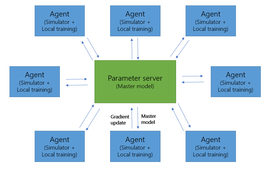
One of the fortunate factors of the training process is that it can be easily parallelized. After a training epoch is over, the environment is totally reset. That means that if we have the computational resources to spin up many machines to run training agents in parallel, we can increase the rate at which we train almost linearly. A simple algorithm that has been proposed by Google is called Downpour Stochastic Gradient Descent (DownpourSGD). The algorithm is simple. A single machine is designated as the “parameter server,” which keeps a master copy of the model. All other nodes continuously run the DQN algorithm as described above until the end of an epoch is reached. Once an epoch is finished, the agent machines will perform a training iteration of the action model and compute the resulting change in model weights (the “gradient.”). This gradient will be sent to the parameter server, who will then simply add the received gradient to the existing model’s weights. Then, it will send out the updated model to the agent machine, who will run the next epoch with the latest model. This process allows the training process to scale out almost indefinitely, leading to a reduction in training time proportional to the number of agent nodes in the system (e.g. if the job takes 1 week on a single machine, then the job will take 1 day on 7 machines). The graphic below summarizes the responsibilities of each of the nodes in the system and the flow of data between the nodes.

experiment_architecture

Transfer Learning

If we have some labeled training data, we can put this to use to drastically cut down on the training time as well. For example, for this problem we may have some combinations of (image) -> (steering angle) from an expert driver. If we have this data, we can begin by setting up a model that is identical to our DQN, aside from the last dense layer (it would have a single scalar output instead of 5). After training this model on our labeled data, we can copy the weights for the first few layers (e.g. the convolutional layers) into the DQN and freeze them. This allows us to drastically reduce training time by starting with a reasonable set of extracted features as well as reducing the number of free parameters for the model. For example, in this problem using pretrained weights pulled training time down from a few days to a few hours!

The Example Code

To go with this post, I have developed a tutorial on The Autonomous Driving Cookbook to solve the problem of learning to steer via Reinforcement Learning. The tutorial has been developed to work with Azure Batch to allow the experiment to scale out and reduce training time. In addition to Batch, the reinforcement learning code can be run locally as well. The code is all in python, so it can be easily modified to try different network architectures and different variations on the training algorithm. Here is a short video of what the model will look like when it finishes training:

car_driving

UPDATE: Based on the work done for this tutorial, we were able to submit a publication to the International Conference for Software Engineering (ICSE)! Here is a link to the paper

Summary

In this post, we applied Q Learning to solve a non-trivial problem: learning to drive an autonomous vehicle. We saw why the Bellman Equation cannot be directly applied in this case to compute the Q values, necessitating a predictive model. We saw some of the tricks that were needed to allow the DQN to converge on a solution, and ended up with an end-to-end example that could be used to drive the vehicle. Since the introduction of the DQN, many additional architectural advancements have been made (such as the “Dueling” Deep Q Network), but even with a simple model, it is possible to get very good results on nontrivial problems.

Autonomous Driving with Deep Reinforcement Learning